This post is inspired by a brief twitter thread between Lee Sharpe and Robby Greer as well as Jonathan Goldberg’s previous post on Open Source Football that adjusts EPA/play for opponent using 10 game rolling windows. The goal of this article is to alter EPA/play by adjusting for opponent as well as to determine the best rolling average window to maximize the predictive power of future game outcomes.
Loading in the data
Let’s start by first reading in play-by-play data from 1999-2020 from @nflfastR.
Methodology
Just as Jonathan did in his post, we will find every team’s weekly EPA/play on offense and defense. Additionally, instead of simply finding total offense and defense EPA/play, we will break it down into passing and rushing EPA/play for offense and defense.
### Get game EPA data
# Offense EPA
epa_data <- nfl_pbp %>%
  dplyr::filter(
    !is.na(epa), !is.na(ep), !is.na(posteam),
    play_type == "pass" | play_type == "run" | penalty == 1, qb_kneel != 1
  ) %>%
  dplyr::group_by(game_id, season, week, posteam, home_team) %>%
  dplyr::summarise(
    off_dropback_pct = mean(qb_dropback == 1),
    off_epa = mean(epa),
    off_pass_epa = mean(epa[qb_dropback == 1]),
    off_rush_epa = mean(epa[qb_dropback == 0]),
    off_epa_n = sum(qb_dropback == 1 | qb_dropback == 0),
    off_pass_epa_n = sum(qb_dropback == 1),
    off_rush_epa_n = sum(qb_dropback == 0),
    .groups = "drop"
  ) %>%
  # Defense EPA
  dplyr::left_join(nfl_pbp %>%
    filter(
      !is.na(epa), !is.na(ep), !is.na(posteam),
      play_type == "pass" | play_type == "run" | penalty == 1, qb_kneel != 1
    ) %>%
    dplyr::group_by(game_id, season, week, defteam, away_team) %>%
    dplyr::summarise(
      def_epa = mean(epa),
      def_dropback_pct = mean(qb_dropback == 1),
      def_pass_epa = mean(epa[qb_dropback == 1]),
      def_rush_epa = mean(epa[qb_dropback == 0]),
      def_epa_n = sum(qb_dropback == 1 | qb_dropback == 0),
      def_pass_epa_n = sum(qb_dropback == 1),
      def_rush_epa_n = sum(qb_dropback == 0),
      .groups = "drop"
    ),
  by = c("game_id", "posteam" = "defteam", "season", "week")
  ) %>%
  dplyr::mutate(opponent = ifelse(posteam == home_team, away_team, home_team)) %>%
  dplyr::select(
    game_id, season, week, home_team, away_team, posteam, opponent,
    off_dropback_pct, off_epa, off_pass_epa, off_rush_epa,
    off_epa_n, off_pass_epa_n, off_rush_epa_n,
    def_epa_n, def_pass_epa_n, def_rush_epa_n,
    def_dropback_pct, def_epa, def_pass_epa, def_rush_epa
  ) %>%
  # Not sure why, but there is one instance where the posteam = ""
  dplyr::filter(posteam != "")
We are going to build our dataset in a very similar manner to what Jonathan did in his post, with a few changes outlined below:
Convert each EPA statistic into a lagging moving average. The lag ensures that we compare a team’s performance against their opponent’s performance up to that point in the season.
Instead of weighting each game equally during the window, we will weight EPA by the number of plays in each game of the window.
Instead of simply converting each statistic into a moving average of the last ten games, we will convert each statistic into a moving average using a dynamic window that ranges from ten games to twenty games (for teams that play in the Super Bowl). In other words, we will use a ten game window to predict the winner of the 11th game, but for say the 15th game, we will use a 14 game window.
Note that for new seasons, this ten game window serves as a prior for each team in a similar manner to Football Outsiders’ weighted DVOA. For example, to predict week 3, we will use a rolling average that includes 8 games from the previous year along with weeks 1 and 2.
We will ignore the 1999 season and only analyze the predictive power of EPA starting with the 2000 season, allowing us to use the 1999 season as a prior.
Finally, the
pracmapackage offers several types of rolling averages, including simple, weighted, running and exponential rolling averages. We will play around with these types of moving averages to see what maximizes predictive power.
If you want to look at all the code for building this dataset, view the source file! Here is the function to compute moving averages based on varying window sizes:
# Function to get moving average of a dynamic window from 10 - 20 games
wt_mov_avg_local <- function(var, weight, window, type, moving = T) {
  if (length(weight) == 1 & weight[1] == 1) {
    weight <- rep(1, length(var))
  }
  if (moving) {
    dplyr::case_when(
      window == 10 ~ pracma::movavg(var * weight, n = 10, type = type) /
        pracma::movavg(weight, n = 10, type = type),
      window == 11 ~ pracma::movavg(var * weight, n = 11, type = type) /
        pracma::movavg(weight, n = 11, type = type),
      window == 12 ~ pracma::movavg(var * weight, n = 12, type = type) /
        pracma::movavg(weight, n = 12, type = type),
      window == 13 ~ pracma::movavg(var * weight, n = 13, type = type) /
        pracma::movavg(weight, n = 13, type = type),
      window == 14 ~ pracma::movavg(var * weight, n = 14, type = type) /
        pracma::movavg(weight, n = 14, type = type),
      window == 15 ~ pracma::movavg(var * weight, n = 15, type = type) /
        pracma::movavg(weight, n = 15, type = type),
      window == 16 ~ pracma::movavg(var * weight, n = 16, type = type) /
        pracma::movavg(weight, n = 16, type = type),
      window == 17 ~ pracma::movavg(var * weight, n = 17, type = type) /
        pracma::movavg(weight, n = 17, type = type),
      window == 18 ~ pracma::movavg(var * weight, n = 18, type = type) /
        pracma::movavg(weight, n = 18, type = type),
      window == 19 ~ pracma::movavg(var * weight, n = 19, type = type) /
        pracma::movavg(weight, n = 19, type = type),
      window == 20 ~ pracma::movavg(var * weight, n = 20, type = type) /
        pracma::movavg(weight, n = 20, type = type)
    )
  } else {
    pracma::movavg(var * weight, n = 10, type = type) /
      pracma::movavg(weight, n = 10, type = type)
  }
}
Analyzing predictive power
First, let’s create a dataset where we use simple moving averages along with a static window of just ten games as a baseline (this is the idea in Jonathan’s post) and compare it with a dataset where we use a simple moving averages along with a dynamic window that ranges from ten to twenty games.
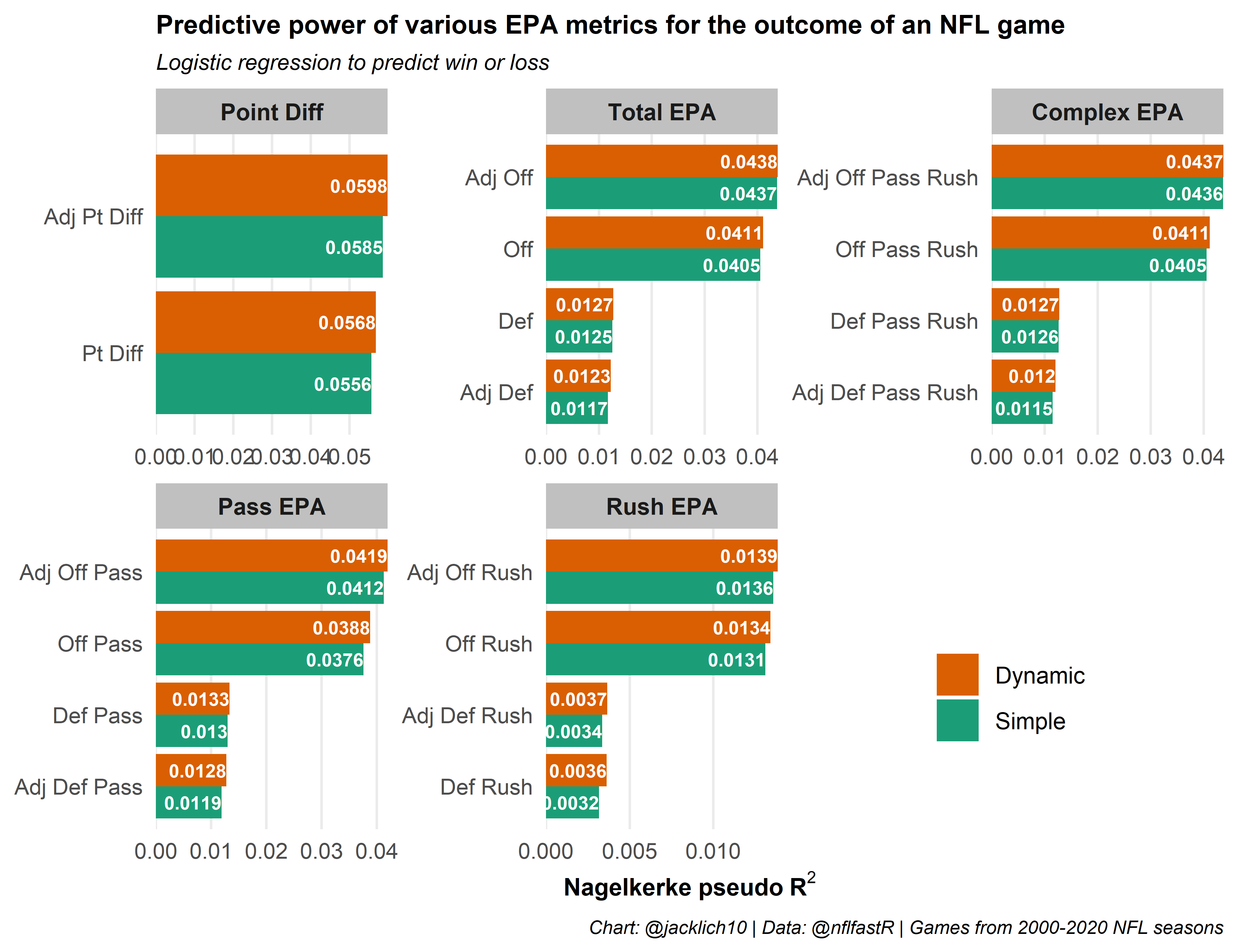
Awesome! It looks like using the dynamic window (which always adds the additional information from all games played during a season) increases the predictive power of EPA/play, rather than using a static window that looks only at a team’s previous ten games.
Note that the “Complex” category combines pass and rush EPA/play together as follows:
\[\text{off_pass_rush_epa} = \text{off_dropback_pct}*\text{off_pass_epa} + (1-\text{off_dropback_pct})*\text{off_rush_epa}\]
In other words, it combines a team’s pass and rush EPA/play into a total EPA/play by weighting them by the percentage of time a team drops back to pass. The difference between this and total EPA/play is that the complex version adjusts pass and rush EPA separately according to the strength of opponent pass and rush EPA, whereas total EPA adjusts based on opponent holistically.
What’s interesting is that adjusting defensive EPA/play for opponent offenses faced actually decreases its predictive power, albeit a very small amount. This finding might provide a little support to the “defenses are simply a product of the offenses they face”, as penalizing or rewarding defenses based on the quality of the offense they face might simply be adding noise. Of course, in general, defensive strength as measured through EPA is much less predictive than offensive strength.
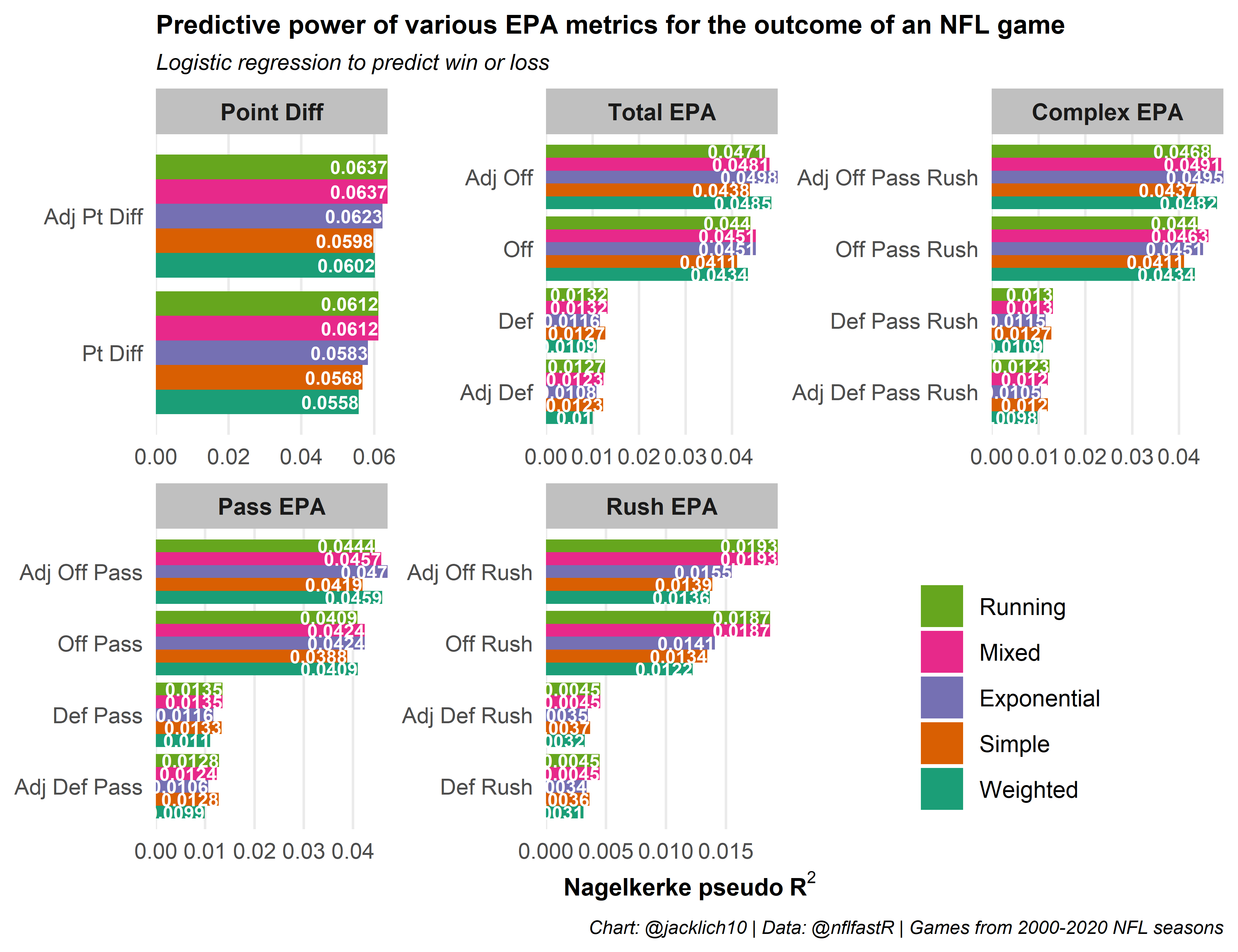
Now that we know that using a dynamic window for the rolling averages works better than a simple static ten game window, let’s play around with different types of moving averages from the pracma package. We will try weighted, running and exponential averages compared to the simple moving averages from above.

There is a lot to take in here, so let’s break it down by category of predictor:
Point Differential: It seems clear that a running moving average of point differential increases its predictive power the most.
Total Offense/Defense EPA: In terms of offensive EPA, an exponential moving average works best (this is primarily driven by passing offense). In terms of defensive EPA, simple or running moving averages work best and it is difficult to discern between the two.
Offense Pass EPA: An exponential moving average best predicts offensive pass EPA.
Defense Pass EPA: Simple and running moving averages do about equally.
Offense/Defense Rush EPA: A running moving average outclasses the other options.
In general, weighting recent performance more heavily increases a metric’s predictive strength. Let’s see if we can’t combine the best types of rolling average for each predictor to generate the best set of predictors for the outcome of a game. We will use a running average for point differential, rushing offense/defense, as well as for passing and total defense and an exponential moving average for offensive pass EPA and total offensive EPA.
So mixing the types of moving averages yields some benefits and some drawbacks. We are able to achieve the maximum level of predictive power for point differential and rushing offense/defense, however passing offense/defense suffers. It appears that when adjusting passing offense for opponent, it is better to use a lagging exponential moving average of opponent defense, yet this lagging exponential moving average of defense significantly decreases the predictive power of defensive EPA. Obviously, more work can be done to play around with different combinations of moving averages, although some improvements could easily be attributed to random noise. For now, let’s use the mixed dataset to explore!
Exploration
If you follow Ben Baldwin on twitter or have visited his awesome website https://rbsdm.com/, you may be familiar with his weekly team tiers scatter plot. Let’s look at the differences between those team tiers (which use unadjusted, cumulative mean EPA) and team tiers using our framework:
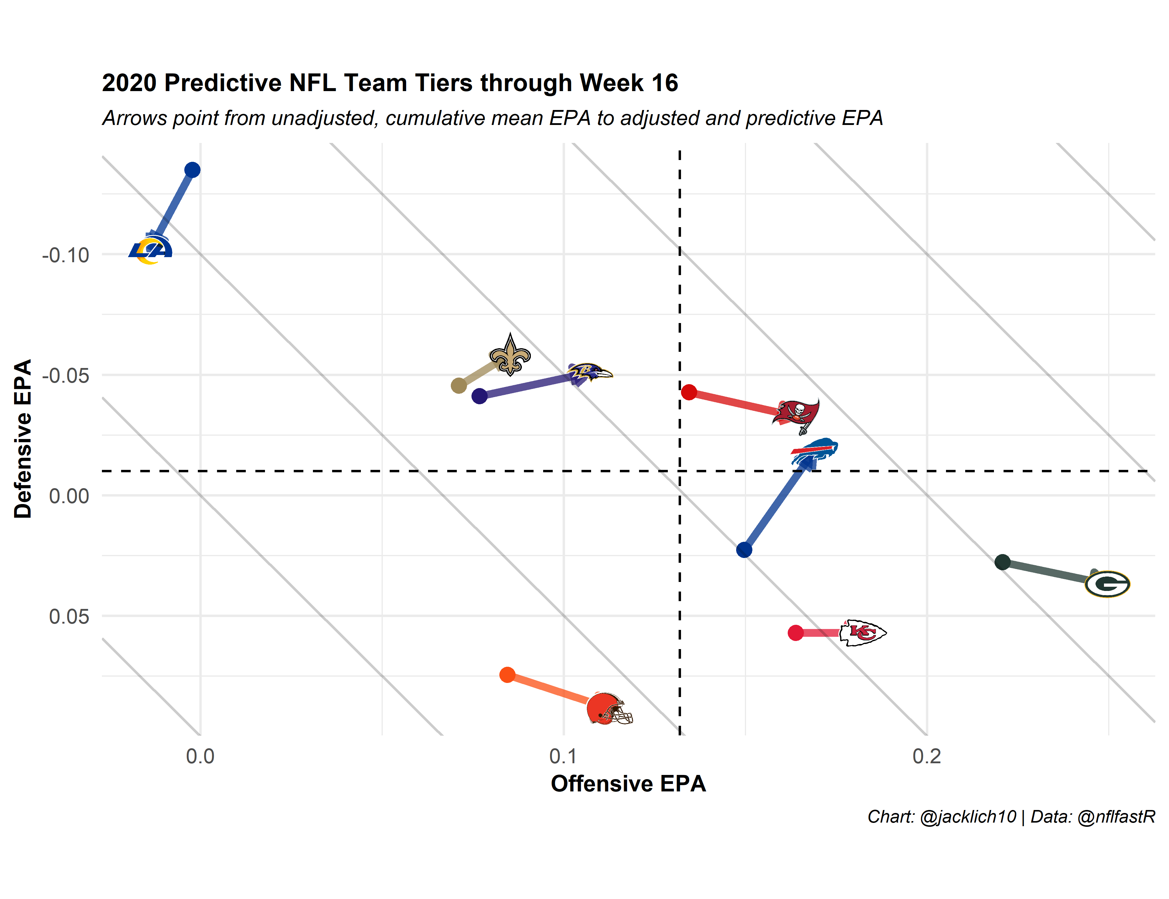
Wow, look at the Bills and Ravens! Everybody thinks the Chiefs are unbeatable, but their path to the Super Bowl seems much more treacherous than last years… We also see that the Rams’ and Steelers’ offenses and defenses have regressed since the beginning of the year.
As a Jets fan, I can’t help but look at the Jets ruining their quest for Trevor Lawrence as the Jags ensure the losing continues! 😢
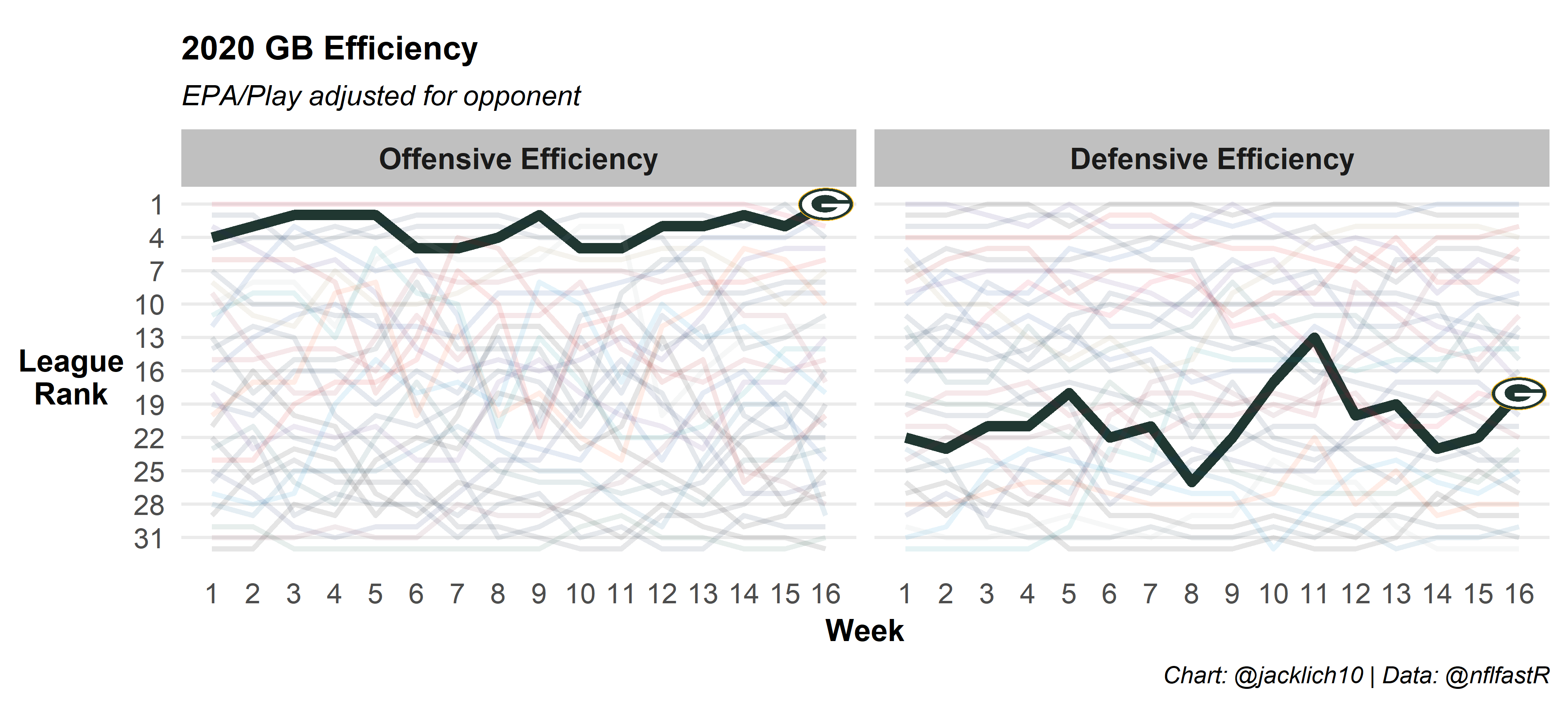
We can also look at a team’s offensive and defensive efficiency over the course of the season using our methodology. Here’s the Chiefs and some AFC competitors:


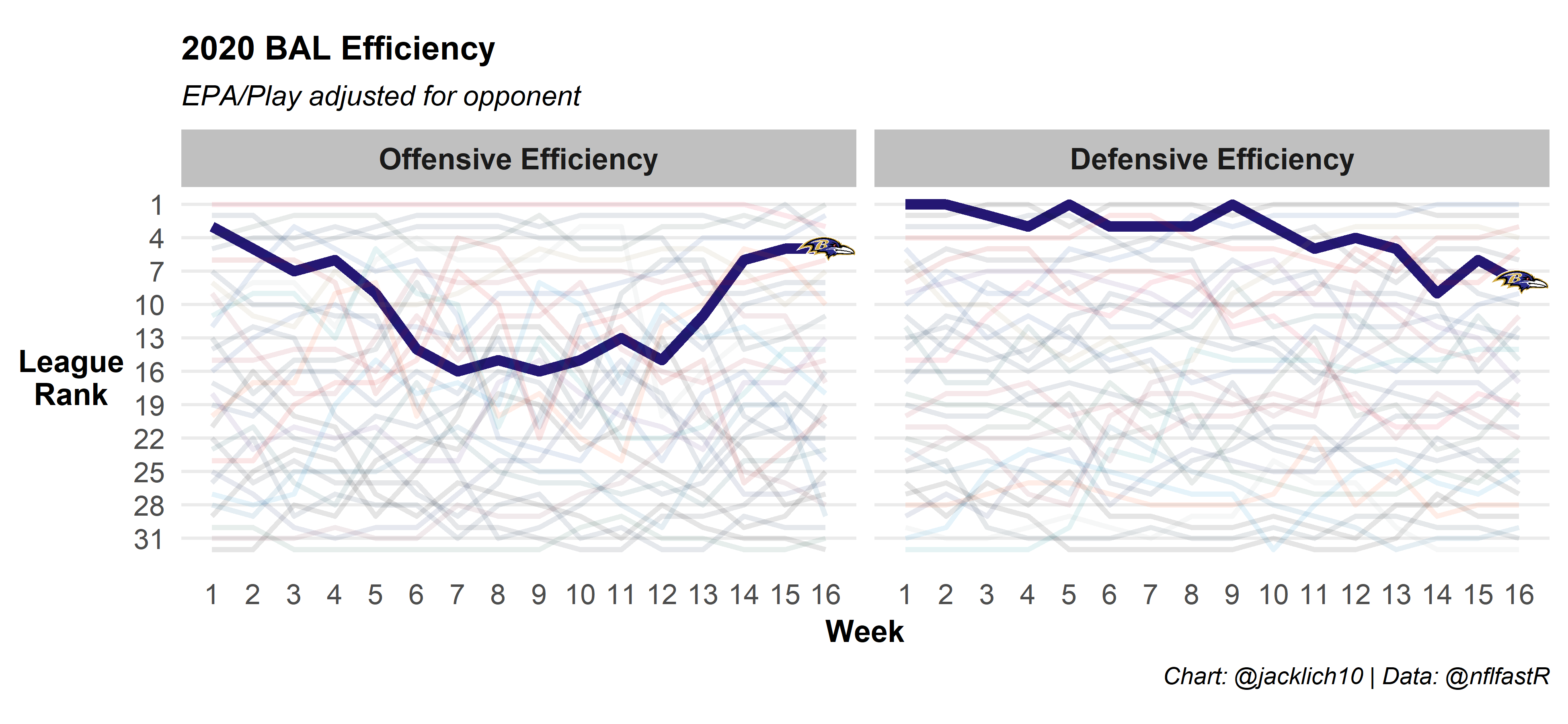
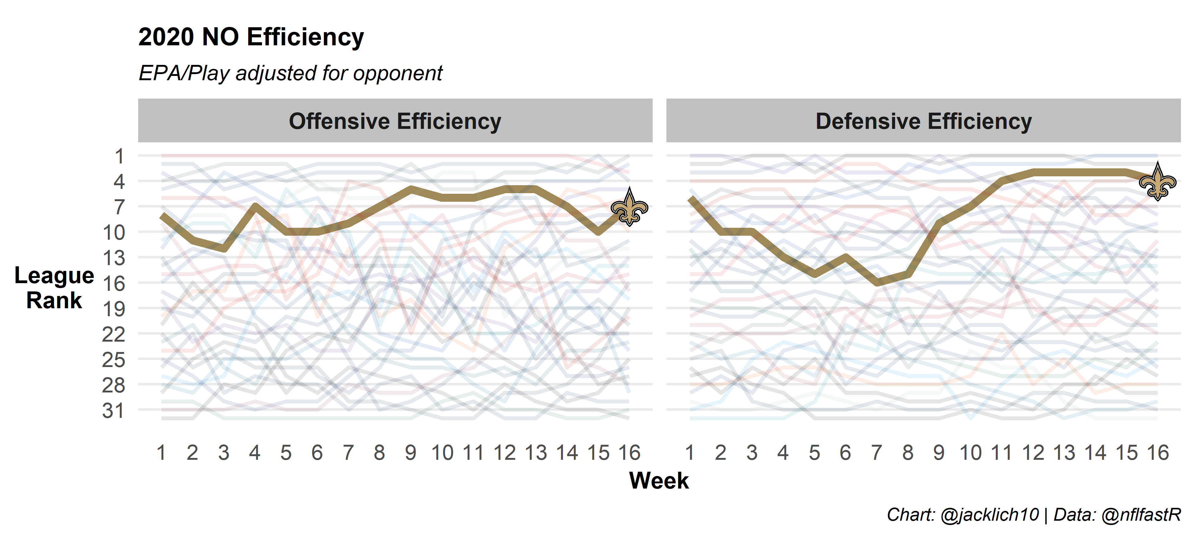
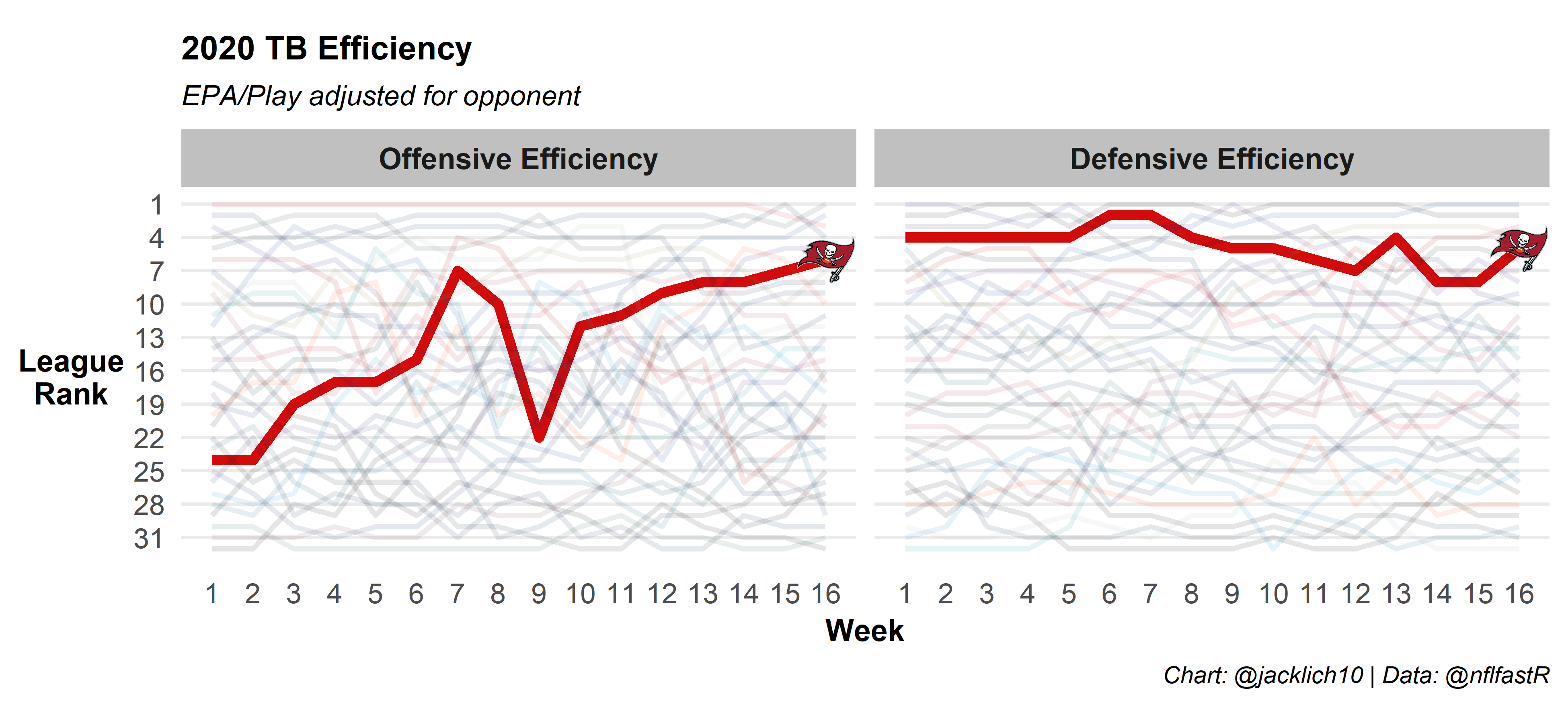
And here’s some NFC competitors:
Final Thoughts
The main objective of this post was to improve the predictiveness of EPA by exploring rolling averages and dynamically moving windows. Certainly, rolling 250 play averages of EPA, for example, can provide important descriptive information. However, as with most predictive measures, this work provides evidence that using the widest window of available data yields the best results. Nonetheless, there are definitely ways to improve this methodology. More work can be done in altering which types of moving averages are used for each facet of play. Additionally, note that the post does not explore weighting EPA for given types of plays. For example, weighting EPA by win probability, increasing the value of EPA on early downs or down-weighting turnovers will probably yield significant increases in its predictive power. It is also somewhat surprising that adjusting pass and rush EPA individually for opponent does not seem to produce much of an advantage, although perhaps a more in-depth technique might yield predictive benefits. Hopefully this analysis is another small iteration in improving EPA as a predictive metric!
Thanks to Sebastian Carl and Ben Baldwin for creating this forum and providing awesome open source football analysis throughout the year, as well as to Jonathan Goldberg, Lee Sharpe and Robby Greer for their inspiration.