Here we are going to take a look at how to adjust a team’s epa per play to the strength of their opponent. This technique will use weekly epa/play metrics, which can ultimately summarize a team’s season-long performance. It is also possible to adjust the epa of individual plays with this process if you are so inclined to do so.
Quick note: the adjustments were inspired by the work done in this paper. It’s a bit technical but a good additional read!
Alright, let’s get into it by first loading up our data!
NFL_PBP <- purrr::map_df(2009:2019, function(x) {
  readr::read_csv(
    glue::glue("https://raw.githubusercontent.com/guga31bb/nflfastR-data/master/data/play_by_play_{x}.csv.gz")
  )
})
With the data loaded, we can finally get down to business by summarizing each team’s weekly epa/play.
library(tidyverse)
epa_data <- NFL_PBP %>%
  dplyr::filter(!is.na(epa), !is.na(ep), !is.na(posteam), play_type == "pass" | play_type == "run") %>%
  dplyr::group_by(game_id, season, week, posteam, home_team) %>%
  dplyr::summarise(
    off_epa = mean(epa),
  ) %>%
  dplyr::left_join(NFL_PBP %>%
    filter(!is.na(epa), !is.na(ep), !is.na(posteam), play_type == "pass" | play_type == "run") %>%
    dplyr::group_by(game_id, season, week, defteam, away_team) %>%
    dplyr::summarise(def_epa = mean(epa)),
  by = c("game_id", "posteam" = "defteam", "season", "week"),
  all.x = TRUE
  ) %>%
  dplyr::mutate(opponent = ifelse(posteam == home_team, away_team, home_team)) %>%
  dplyr::select(game_id, season, week, home_team, away_team, posteam, opponent, off_epa, def_epa)
Now we can get into the fun part: adjusting a team’s epa/play based on the strength of the opponent they are up against.
- We are going to reframe each team’s epa/play as a team’s weekly opponent.
- We are going to convert each statistic into a moving average of the last ten games — this decision was based on this research and this model — and lag that statistic by one week. The lag is important because we need to be comparing a team’s weekly performance against their opponent’s average performance up to that point in the season.
- We are going to join the data back to the epa_dataset.
# Construct opponent dataset and lag the moving average of their last ten games.
opponent_data <- epa_data %>%
  dplyr::select(-opponent) %>%
  dplyr::rename(
    opp_off_epa = off_epa,
    opp_def_epa = def_epa
  ) %>%
  dplyr::group_by(posteam) %>%
  dplyr::arrange(season, week) %>%
  dplyr::mutate(
    opp_def_epa = pracma::movavg(opp_def_epa, n = 10, type = "s"),
    opp_def_epa = dplyr::lag(opp_def_epa),
    opp_off_epa = pracma::movavg(opp_off_epa, n = 10, type = "s"),
    opp_off_epa = dplyr::lag(opp_off_epa)
  )

# Merge opponent data back in with the weekly epa data
epa_data <- epa_data %>%
  left_join(
    opponent_data,
    by = c("game_id", "season", "week", "home_team", "away_team", "opponent" = "posteam"),
    all.x = TRUE
  )
Don’t fret that the opponent’s epa columns will have NAs in the first week. You simply can’t lag from the first observation.
The final piece of the equation needed to make the adjustments is the league mean for epa/play on offense and defense. We need to know how strong the opponent is relative to the average team in the league.
epa_data <- epa_data %>%
  dplyr::left_join(epa_data %>%
    dplyr::filter(posteam == home_team) %>%
    dplyr::group_by(season, week) %>%
    dplyr::summarise(
      league_mean = mean(off_epa + def_epa)
    ) %>%
    dplyr::ungroup() %>%
    dplyr::group_by(season) %>%
    dplyr::mutate(
      league_mean = lag(pracma::movavg(league_mean, n = 10, type = "s"), ) # We lag because we need to know the league mean up to that point in the season
    ),
  by = c("season", "week"),
  all.x = TRUE
  )
Finally, we can get to adjusting a team’s epa/play. We’ll create an adjustment measure by subtracting the opponent’s epa/play metrics from the league mean. Then we add the adjustment measure to each team’s weekly performance.
# Adjust EPA
epa_data <- epa_data %>%
  dplyr::mutate(
    off_adjustment_factor = ifelse(!is.na(league_mean), league_mean - opp_def_epa, 0),
    def_adjustment_factor = ifelse(!is.na(league_mean), league_mean - opp_off_epa, 0),
    adjusted_off_epa = off_epa + off_adjustment_factor,
    adjusted_def_epa = def_epa + def_adjustment_factor,
  )
We’re done! You can now view each team’s epa/play adjusted for their strength of schedule. Let’s check out how different the league looks by comparing unadjusted epa to adjusted epa stats.
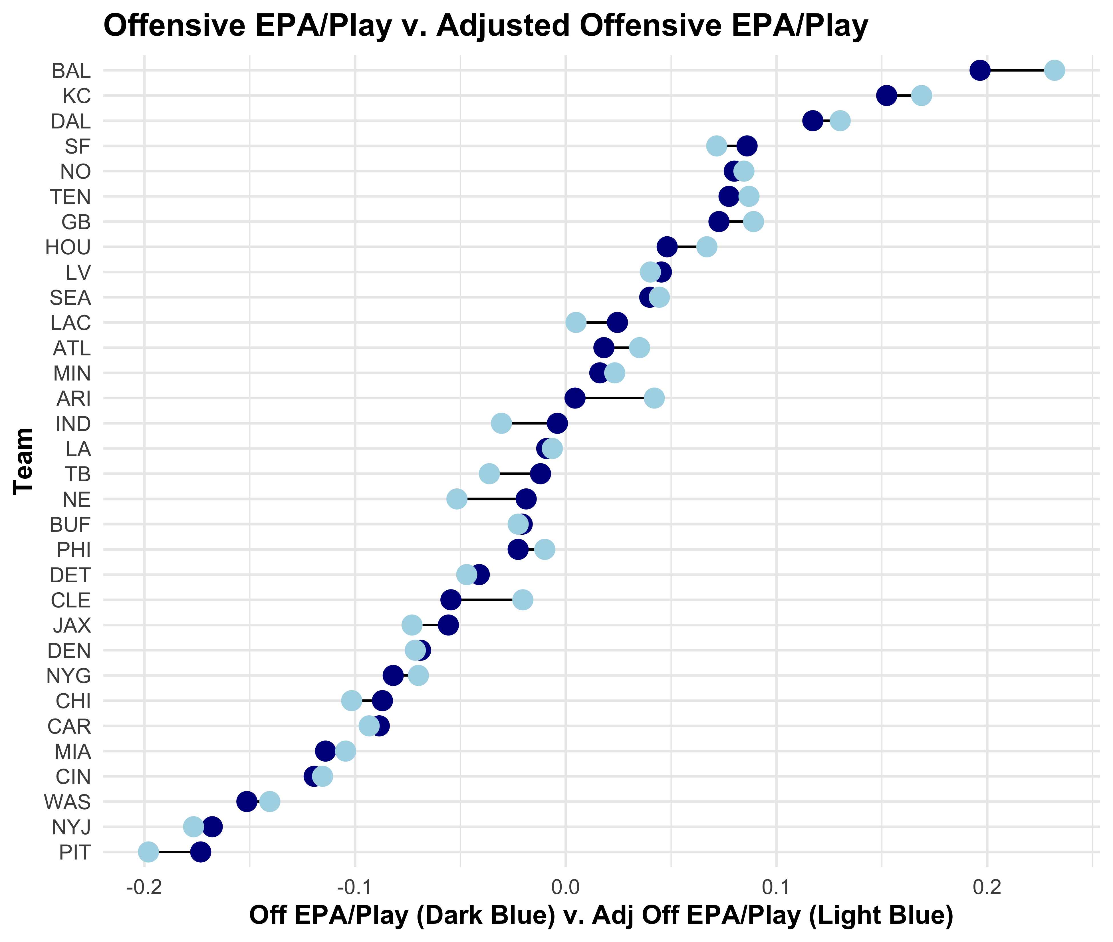
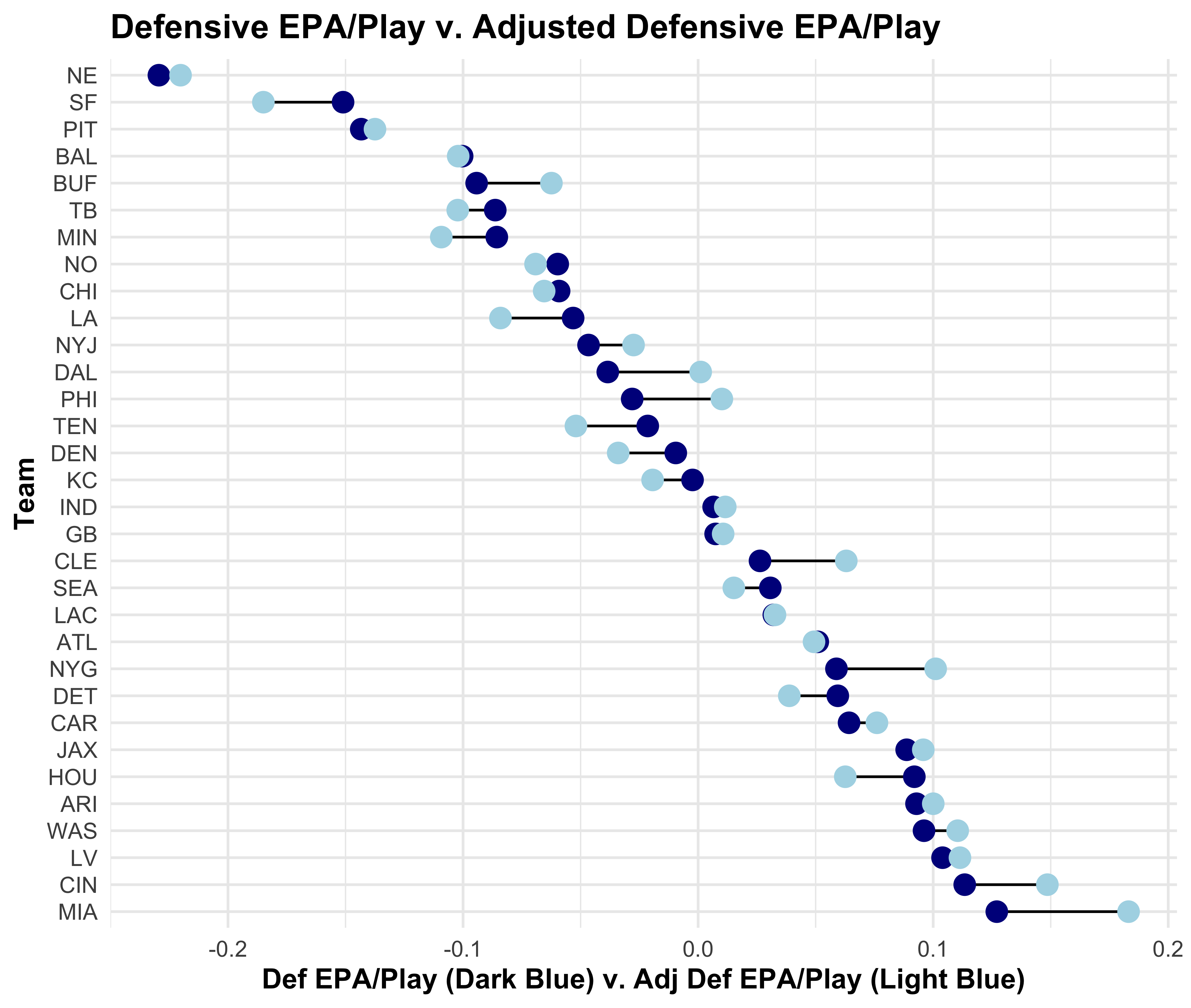
Above, you can see that some teams are revealed to be stronger after adjusting their epa/play while other teams appear to be weaker. We can use these adjustments to make more accurate predictions of individual NFL games.
Here, each metrics are used in separate glm models to predict the outcome of games from the past two seasons. Their accuracy is below.
[1] "Adjusted EPA Accuracy"
[1] 0.6404494
[1] "Normal EPA Accuracy"
[1] 0.6348315There is a slight edge to the adjusted EPA model. Its a solid start but there is more work to be done in finding the best version on epa/play.
- There is good work being done on properly weighting epa on a given type of play. For instance, DVOA is a does well in predicting future team performance because the downweight the impact of interceptions in their metric. More work can be done to properly weight epa based on its play type!
- It is possible to make these adjustments at the individual play level and with more specificity. For instance, you could adjust run plays based on the team’s run defense rather than adjusting the entire offense to the team’s entire defense. I think more work should be done to determine if these more detailed techniques can improve the predictiveness of the stat.
- There may be other ways to construct epa/play that improve its strength as a predictor The paper that inspired this article uses the solution of an optimization problem to construct a team’s true offensive epa/play and defensive epa/play. Perhaps a moving averaged should be eschewed in favor of a technique that more properly accounts for common regression to the mean over the offseason.
Thanks to Sebastian Carl and Ben Baldwin for setting this forum up! I can’t wait to see others’ works and improvements to my own make its way on here.