Intro:
A few years ago, Bill Petti posted a great article on FanGraphs describing hitter volatility and how it can be quantified via Gini coefficients. Petti wrote that volatility is how a player distributes their overall season performance (as measured by wRC in his case) throughout the season on a game by game basis. This is opposed to streakiness which is related to clustering of good and bad performances over the course of a season. To quantify a hitters volatility, he proposed the usage of a Gini coefficient. Typically Gini coefficients are used to evaluate the wealth distribution in countries (0-1 scale where higher values indicate less equal distribution of wealth). In the case of football, a Gini coefficient can tell us how each individual quarterback distributes their cumulative season EPA (passes, rushes, penalties) on a game by game basis (includes playoffs).
In this post, I follow a similar methodology to Petti’s original work to calculate a quarterback’s volatility by season. In addition, I create a “Volatility Over Expected (VOLoe)” GAM model to evaluate a QB’s volatility within the context of their season EPA and total opportunities (passes, rushes, penalties).
Data Prep and Packages
This post uses NFLfastR quarterback data from 1999 to 2020. The full data prep process can be found on my GitHub (just a long loop that loads the data, adds rosters so we can filter for only QB’s, and adding team colors). Some of the notable assumptions in the data cleaning process are: 1. Games where QB x is involved in less than 5 plays (passes, rushes, penalties) are removed from that QB’s history. This is under the assumption that if QB x was involved in so few plays, they were injured or rested. Since the gini coefficient doesn’t consider the amount of plays in a game, this method protects the gini score from being inflated by very low opportunity, low EPA games. 2. Filtered for QB’s who threw greater than 250 passes in a season.
#packages
library(dplyr)
library(ggcorrplot)
library(ggplot2)
library(gt)
library(mgcv)
library(nflfastR)
library(readr)
library(tidyverse)

#load data
DF <- read_rds("VOL_DF.rds") %>%
  filter(
    plays >= 10,#remove any games where QB was involved in less than 10 plays
    season_plays >= 250) #filter for greater than 250 attempts
Gini Coefficient Calculation & Analysis
To calculate each QB’s gini coefficient, we can use the same function created in Petti’s article. A typical gini calculation can’t be used with EPA because of negative EPA values, thus the modified gini method has to be used.
#Gini coefficient function to handle negative EPA
Gini_Function <- function(Y) {

  Y <- sort(Y)

  N <- length(Y)

  u_Y <- mean(Y)

  top <- 2/N^2 * sum(seq(1,N)*Y) - (1/N)*sum(Y) - (1/N^2) * sum(Y)

  min_T <- function(x) {

    return(min(0,x))

  }

  max_T <- function(x) {

    return(max(0,x))

  }

  T_all <- sum(Y)

  T_min <- abs(sum(sapply(Y, FUN = min_T)))

  T_max <- sum(sapply(Y, FUN = max_T))

  u_P <- (N-1)/N^2*(T_max + T_min)

  return(top/u_P)

}

#calculate gini scores for our QBs
pbp_QBs_gini <- DF %>%
  select(id, season, Total_EPA) %>%
  na.omit() %>%
  aggregate(Total_EPA ~ id + season, data = ., FUN = "Gini_Function") %>%
  rename("VOL" = "Total_EPA")%>%
  left_join(DF, by = c("id", "season")) %>%
  filter(VOL != "NaN")

#remove extra data
rm(DF)
rm(Gini_Function)
Applying the function to our data frame yields a gini score for each quarterback season since 1999 (minimum 250 throws in given season). We can then plot a QB’s volatility and EPA/Play in the 2020 season. Lower volatility is better, meaning up and to the right is best.
#group up each QB & season
QBs_Grouped <- pbp_QBs_gini %>%
  group_by(
    id,
    season
  ) %>%
  #group by each QB to see their VOL on a season by season basis
  summarize(
    name  = unique(name),
    color = unique(team_color),
    VOL   = unique(VOL),
    EPA_play = unique(Season_EPA),
    Plays = sum(plays)
  ) %>%
  ungroup()

#check who the least volatile, highest EPA/Play QB's were in 2020
Data_2020 <- QBs_Grouped %>%
  filter(season == 2020)

Data_2020 %>%
  ggplot(aes(x = EPA_play, y = VOL)) +
  geom_point(colour = "black", shape=21, size = 3,
             aes(x = EPA_play, y = VOL), fill = Data_2020$color, alpha = .75)+
  theme_light() +
  geom_abline(slope = -1.5, intercept = c(-1,-.8, -.6, -.4, -.2, 0),
              alpha = .2)+
  theme(plot.title = element_text(color="black", size=8, face="bold"))+
  theme(plot.title = element_text(size = 10, face = "bold"),
        plot.subtitle = element_text(size = 8))+
  theme(plot.background = element_rect(fill = "gray97"))+
  theme(panel.background = element_rect(fill = "gray97"))+
  labs(title = "Good Quarterbacks are Consistent While Bad Quarterbacks are Volatile",
       subtitle = "Relationship Between Volatility and EPA/Play (2020) - Minimum 250 Plays",
       caption = "Plot: PatriotsStatsR, Data: NFLFastR")+
  ylab("Volatility")+
  xlab("EPA/Play")+
  geom_hline(yintercept = mean(Data_2020$VOL) , linetype = "dashed") +
  geom_vline(xintercept = mean(Data_2020$EPA_play), linetype = "dashed") +
  ggrepel::geom_text_repel(aes(label=name), box.padding = 0.4) +
  scale_y_reverse()
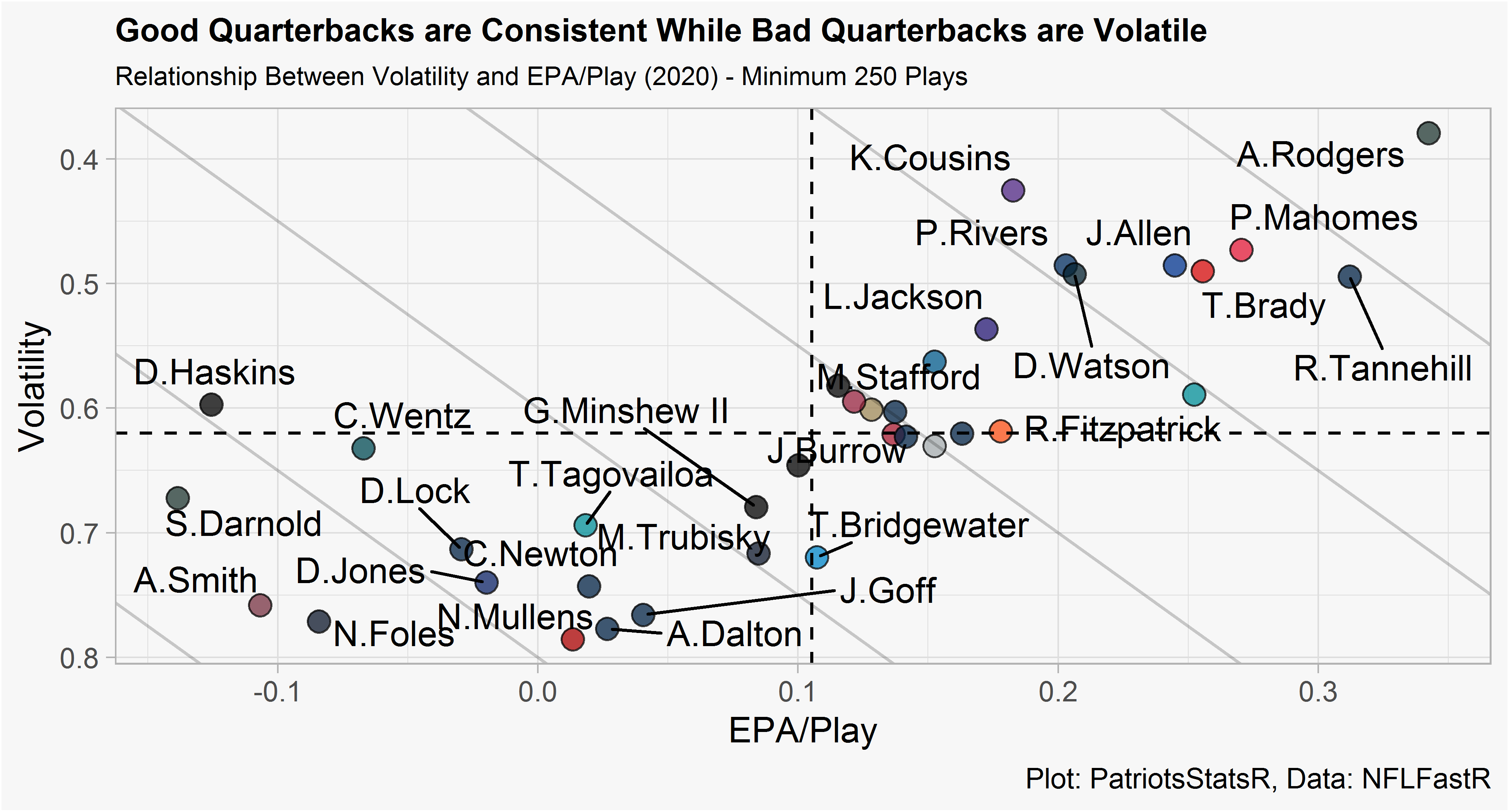
This isn’t too surprising, good quarterbacks (as measured by EPA/Play) are consistent while middle of the pack QB’s tend to be the most volatile. Once we reach the worst QB’s (Wentz, Haskins, Darnold) those players tend to be consistently bad. Essentially, the relationship between EPA/Play and volatility is a parabola shape.
This plot also provides perspective on QB’s who have a similar EPA/Play but have very different levels of volatility. For example, Wentz (-0.06 EPA/Play) and Foles (-0.08 EPA/Play). If a decision maker was in the unfortunate position of deciding between these two below average QB’s, they could possibly prefer the volatile QB (Foles, who has a chance of a great game) over a low volatility QB (Wentz, who is consistently mediocre).
Volatility Over Expected
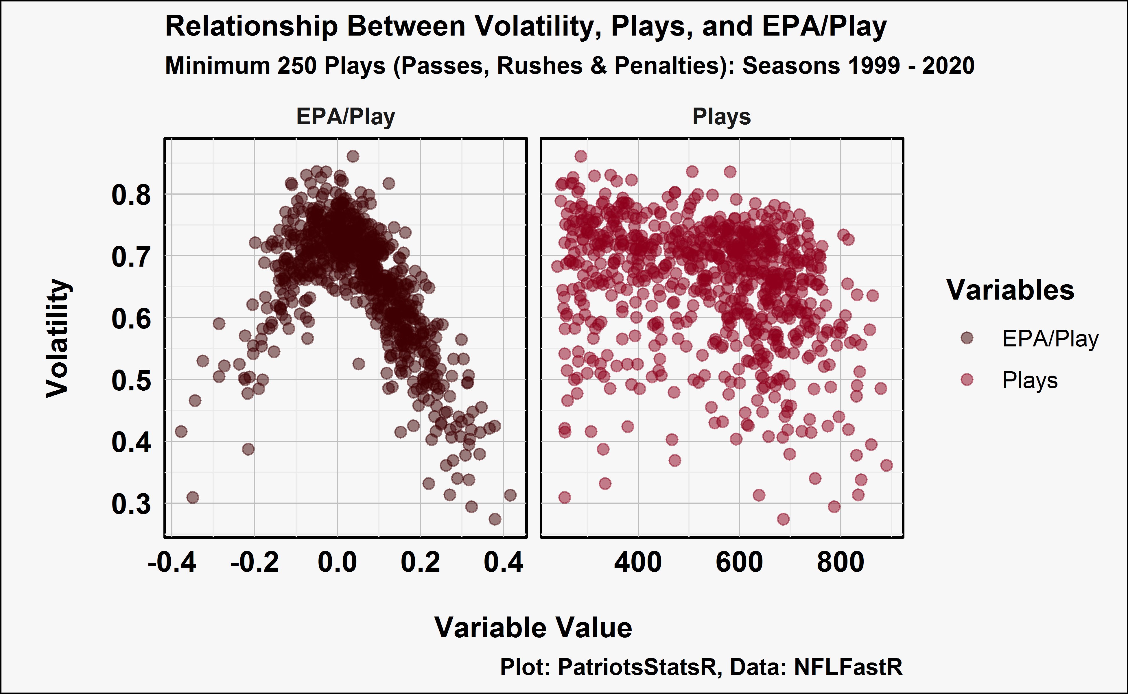
VOL tells a simple story but it doesn’t tell us how much more volatile a QB was given their EPA. E.g. Ryan Tannehill had a 0.31 EPA/Play and a volatility of 0.45, was this more volatile than expected given his performance? We can built a Generalized Additive Model (GAM) with MGCV that includes variables that correlate with VOL. The two variables that most correlate with VOL are EPA/Play & Total Plays.
#create melted data frame of plays & EPA/Play
model_1_data_melted <- QBs_Grouped %>%
  rename("EPA/Play" = "EPA_play") %>%
  gather(key = feature, value = value, -VOL) %>%
  filter(feature %in% c("EPA/Play", "Plays")) %>%
  mutate(value = as.numeric(value), feature = factor(feature))

#color palette from Petti
gini_palette <- c('#3E0002', '#8e001c', '#D87F83', '#969696', '#636363', '#252525')

#plot
model_1_data_melted %>%
  ggplot(aes(value, VOL)) +
  geom_point(aes(color = feature), size = 2, alpha = .5) +
  facet_wrap(~feature, scales = "free_x") +
  xlab("\nVariable Value") +
  ylab("\nVolatility\n") +
  theme_minimal(base_size = 12, base_family = "cairo") %+replace%
  theme(
    panel.border = element_blank(),
    panel.background = element_blank(),
    panel.grid.major = element_line(color='#BFBFBF', size=.25),
    axis.title = element_text(face='bold', hjust=.5, vjust=0),
    axis.text = element_text(color='black')
  ) +
  theme(plot.title = element_text(color="black", size=8, face="bold"))+
  coord_cartesian(clip = "off") +
  theme(plot.title = element_text(size = 12, face = "bold"),
        plot.subtitle = element_text(size = 10))+
  theme(plot.background = element_rect(fill = "gray97"))+
  theme(panel.background = element_rect(fill = "gray97"))+
  labs(title = "Relationship Between Volatility, Plays, and EPA/Play",
       subtitle = "Minimum 250 Plays (Passes, Rushes & Penalties): Seasons 1999 - 2020",
       caption = "Plot: PatriotsStatsR, Data: NFLFastR")+
  scale_color_manual(values = gini_palette, "Variables") +
  theme(title = element_text(face = "bold"),
        axis.text = element_text(face = "bold"),
        strip.text.x = element_text(face = "bold"))
And then we can built the model, I tried a few variations but the model with a 9 knot cubic smoothing spline on EPA/Play performed best.
#Build expected VOL model that controls for EPA & Plays
Modeling_Data <- QBs_Grouped %>%
  select(
    VOL,
    EPA_play,
    Plays
  )

#training test split
set.seed(2018)
df    <- sample(nrow(Modeling_Data), nrow(Modeling_Data) * .7)
train <- Modeling_Data[df,]
test  <- Modeling_Data[-df,]

#tried a few models, GAM performed best
#fit model after trying a few different combos
model1 <- mgcv::gam(VOL ~ s(EPA_play, k = 9, bs="cr") + Plays, data = train)

#check again
mgcv::gam.check(model1, k.rep=1000) #K & EDF are not close, p is no longer significant
Method: GCV   Optimizer: magic
Smoothing parameter selection converged after 4 iterations.
The RMS GCV score gradient at convergence was 4.962146e-09 .
The Hessian was positive definite.
Model rank =  10 / 10

Basis dimension (k) checking results. Low p-value (k-index<1) may
indicate that k is too low, especially if edf is close to k'.

             k' edf k-index p-value
s(EPA_play) 8.0 4.7 1.02 0.69summary(model1) #0.75 adjusted r squared
Family: gaussian
Link function: identity

Formula:
VOL ~ s(EPA_play, k = 9, bs = "cr") + Plays

Parametric coefficients:
              Estimate Std. Error t value Pr(>|t|)
(Intercept)  6.892e-01  9.293e-03  74.170  < 2e-16 ***
Plays       -6.668e-05  1.671e-05  -3.991 7.53e-05 ***
---
Signif. codes:  0 '***' 0.001 '**' 0.01 '*' 0.05 '.' 0.1 ' ' 1

Approximate significance of smooth terms:
              edf Ref.df   F p-value
s(EPA_play) 4.704  5.597 238  <2e-16 ***
---
Signif. codes:  0 '***' 0.001 '**' 0.01 '*' 0.05 '.' 0.1 ' ' 1

R-sq.(adj) =  0.748   Deviance explained = 75.1%
GCV = 0.0027458  Scale est. = 0.0027109  n = 527
#check rmse
fit_1 <- predict(model1, test)
model_1_res_act <- data.frame(actuals = test$VOL, predicted = fit_1) %>%
mutate(errors = predicted - actuals)
rmse <- function(df) {
rmse <- sqrt(mean((df$actuals-df$predicted)^2))
rmse
}
rmse(model_1_res_act) #.05 rmse
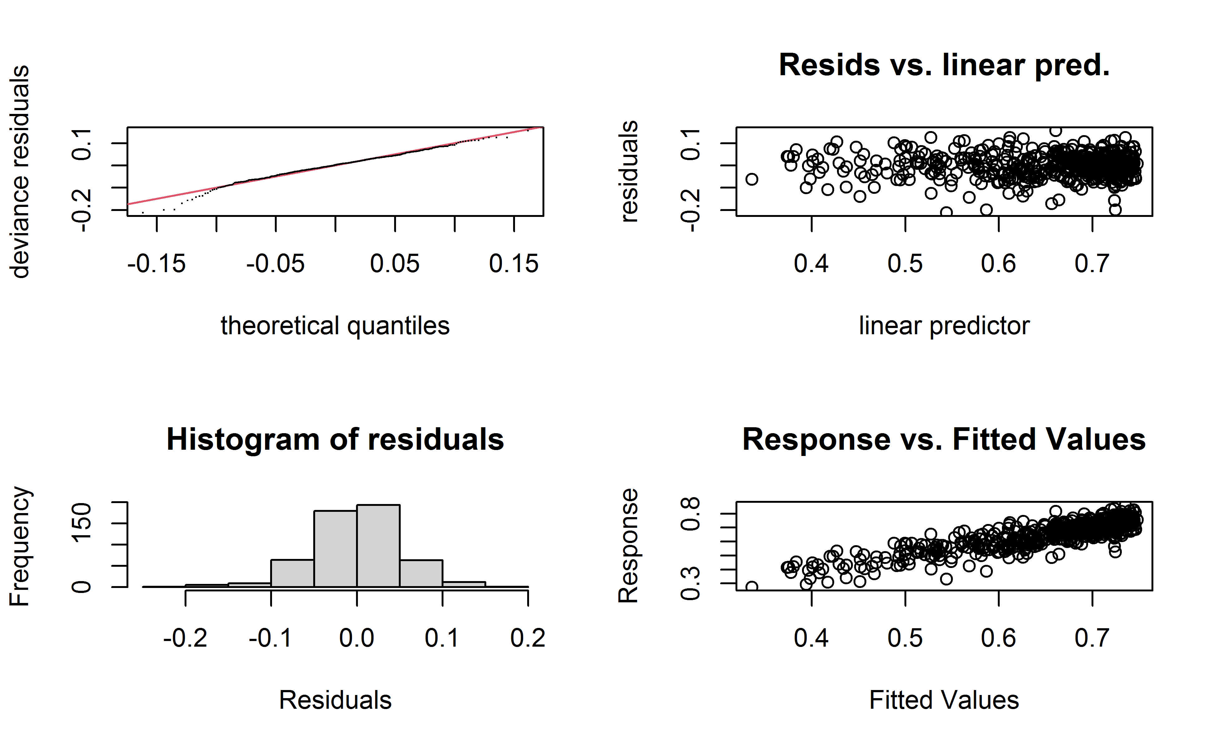
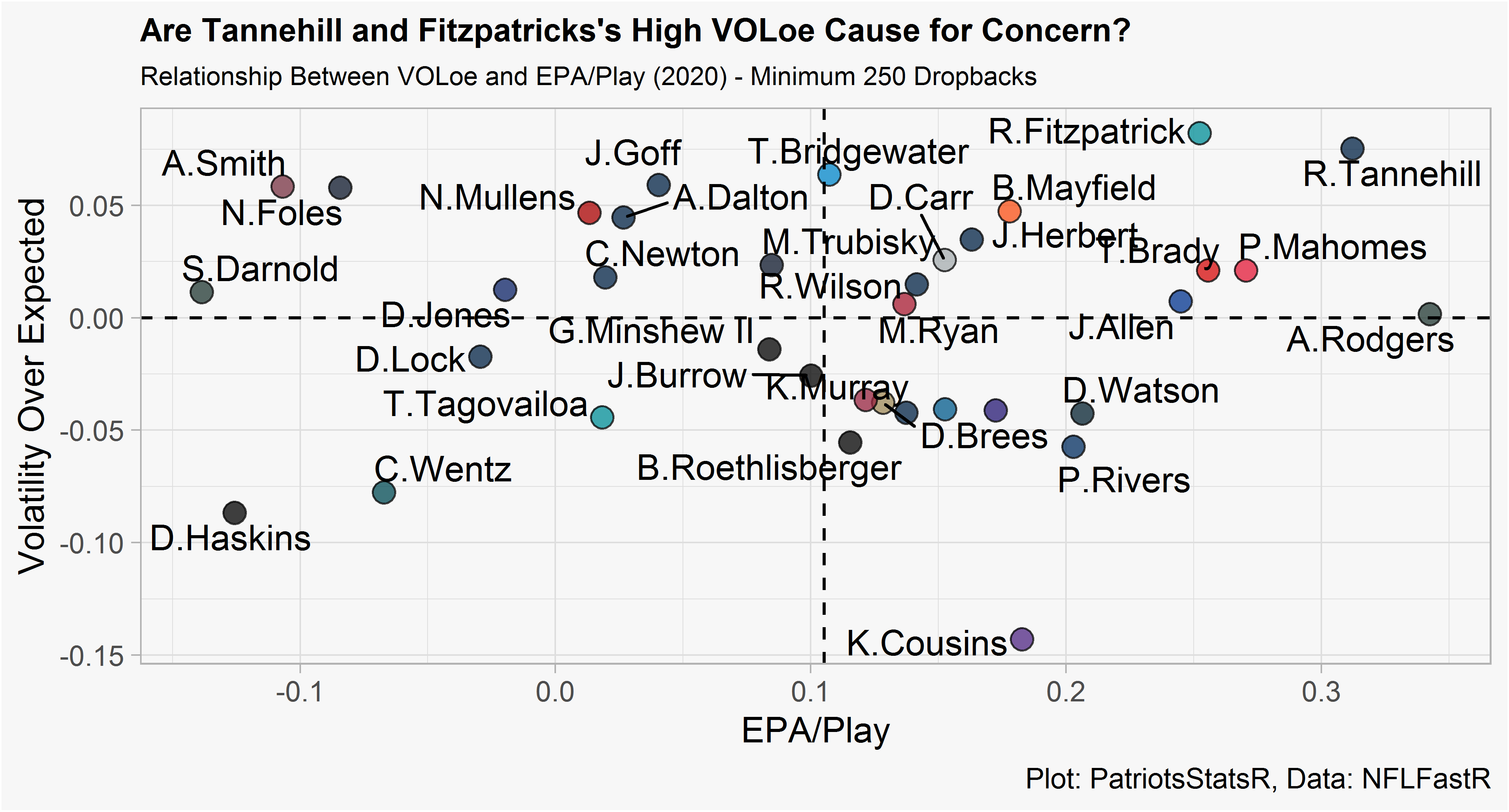
[1] 0.04983998The model has an adjusted R squared of .75, an RMSE of .05, and the GAM check diagnostics pass the smell test. After fitting the model to our data, we can re-plot 2020 QB EPA/Play and VOL over expected. VOLoe values slightly off 0 (Allen, Mahomes, Brady) shouldn’t be cause for concern, instead they should be interpreted as about right where expected. The primary usage of VOLoe should be in detecting significantly higher or lower VOLoe values. Higher VOLoe is worse and represents a more volatile than expected season.
#fit model to actual data
fit_all <- data_frame(predicted = predict(model1, QBs_Grouped))
fit_values <- cbind(QBs_Grouped, fit_all) %>%
  mutate(VOLoe = VOL - predicted)

rm(model1)
rm(fit_all)
rm(model_1_res_act)
rm(test)
rm(train)
rm(Modeling_Data)
rm(df)
rm(fit_1)
rm(model1)
rm(QBs_Grouped)
rm(rmse)

#examine 2020 QBs after controlling for factors in model
fit_2020 <- fit_values %>%
  filter(season == 2020)

fit_2020 %>%
  ggplot(aes(y = VOLoe, x = EPA_play)) +
  geom_point(colour = "black", shape=21, size = 3,
             aes(y = VOLoe, x = EPA_play), fill = fit_2020$color, alpha = .75)+
  theme_light() +
  theme(plot.title = element_text(color="black", size=8, face="bold"))+
  theme(plot.title = element_text(size = 10, face = "bold"),
        plot.subtitle = element_text(size = 8))+
  theme(plot.background = element_rect(fill = "gray97"))+
  theme(panel.background = element_rect(fill = "gray97"))+
  labs(title = "Are Tannehill and Fitzpatricks's High VOLoe Cause for Concern?",
       subtitle = "Relationship Between VOLoe and EPA/Play (2020) - Minimum 250 Dropbacks",
       caption = "Plot: PatriotsStatsR, Data: NFLFastR")+
  ylab("Volatility Over Expected")+
  xlab("EPA/Play")+
  geom_hline(yintercept = 0 , linetype = "dashed") +
  geom_vline(xintercept = mean(fit_2020$EPA_play), linetype = "dashed") +
  ggrepel::geom_text_repel(aes(label=name), box.padding = 0.2)
rm(fit_2020)
Most quarterbacks were close to their predicted level of volatility. Two QB’s that particularly stick out are Fitzpatrick and Tannehill, both performed well but had high volatility over expected scores. A quick investigation of QB’s who had a similar high level of EPA/Play and VOL over expected could perhaps provide insight into if we should be skeptical of this profile.
#find QBs with 85th percentile or greater EPA & VOL
quantile(fit_values$EPA_play, probs = c(0.85)) #.18
      85%
0.1781728 85%
0.04765702 #filter for QBs that fit those conditions
outlier_qbs <- fit_values %>%
filter(EPA_play >= .178, VOLoe >= .05) %>%
mutate(outlier = 1) %>%
select(id,
season,
outlier)
#join data and create table
fit_values %>%
left_join(outlier_qbs, by = c("id", "season")) %>%
group_by(id) %>%
#create indicator that will allow us to filter out QBs without season of interest
mutate(outlier = mean(outlier, na.rm = TRUE)) %>%
ungroup() %>%
filter(outlier != "NaN") %>%
#create summary columns
mutate(
outlier = ifelse(EPA_play >= .178 & VOLoe >= .05, 1, 0), #mark outliers
VOLoe_prior = lag(VOLoe),
follower = lag(outlier),
prior_season = lag(season),
EPA_prior = round(lag(EPA_play), digits = 3),
EPA_diff = round(EPA_play - lag(EPA_play), digits = 3),
EPA_play = round(EPA_play, digits = 3)) %>%
filter(follower == 1) %>%
select(
name,
season,
prior_season,
VOLoe_prior,
EPA_prior,
EPA_play,
EPA_diff
) %>%
rename("VOLoe Prior Season" = "VOLoe_prior") %>%
rename("EPA/Play Prior Season" = "EPA_prior") %>%
rename("EPA/Play Next Season" = "EPA_play") %>%
rename("Change in EPA" = "EPA_diff") %>%
arrange(desc(season)) %>%
filter(prior_season + 1 == season) %>%
arrange(desc(season)) %>%
gt()
| name | season | prior_season | VOLoe Prior Season | EPA/Play Prior Season | EPA/Play Next Season | Change in EPA |
|---|---|---|---|---|---|---|
| D.Prescott | 2020 | 2019 | 0.05301281 | 0.197 | 0.137 | -0.060 |
| L.Jackson | 2020 | 2019 | 0.05003333 | 0.276 | 0.172 | -0.103 |
| D.Brees | 2019 | 2018 | 0.10650383 | 0.303 | 0.184 | -0.119 |
| M.Trubisky | 2019 | 2018 | 0.05707277 | 0.181 | -0.032 | -0.213 |
| D.Watson | 2018 | 2017 | 0.10174379 | 0.220 | 0.123 | -0.097 |
| R.Wilson | 2016 | 2015 | 0.12598953 | 0.212 | 0.093 | -0.119 |
| N.Foles | 2014 | 2013 | 0.06624689 | 0.280 | 0.012 | -0.268 |
| P.Rivers | 2012 | 2011 | 0.08539519 | 0.183 | 0.018 | -0.166 |
| M.Vick | 2011 | 2010 | 0.05385099 | 0.189 | 0.106 | -0.083 |
| D.Brees | 2010 | 2009 | 0.13467862 | 0.298 | 0.138 | -0.161 |
| P.Manning | 2009 | 2008 | 0.06238581 | 0.225 | 0.288 | 0.063 |
| P.Rivers | 2009 | 2008 | 0.09014322 | 0.241 | 0.319 | 0.078 |
| T.Romo | 2008 | 2007 | 0.05295818 | 0.222 | 0.051 | -0.172 |
| P.Manning | 2007 | 2006 | 0.07383574 | 0.237 | 0.259 | 0.021 |
| T.Romo | 2007 | 2006 | 0.10809212 | 0.202 | 0.222 | 0.020 |
| P.Manning | 2006 | 2005 | 0.07194718 | 0.347 | 0.237 | -0.109 |
| B.Roethlisberger | 2006 | 2005 | 0.08175888 | 0.316 | 0.023 | -0.293 |
| D.Brees | 2005 | 2004 | 0.07269145 | 0.314 | 0.136 | -0.178 |
| T.Green | 2004 | 2003 | 0.11238382 | 0.187 | 0.240 | 0.053 |
| P.Manning | 2004 | 2003 | 0.08439443 | 0.233 | 0.416 | 0.183 |
| R.Gannon | 2001 | 2000 | 0.07694551 | 0.194 | 0.183 | -0.011 |
Very small sample size disclaimer but most QB’s with this profile experienced a decrease in their EPA/Play the following season (-.08 average decrease in EPA/Play). It’s difficult to know if this is because of a high VOLoe in the prior season or because it is difficult to maintain an elite level of EPA. This does align with some of skepticism people have about Tannehill and Fitzpatrick though.
Other Questions to Answer
There are a lot of questions related to volatility that come to mind, but for the sake of brevity I will touch upon one that immediately comes to mind: does volatility of VOLoe change with a QB’s age? We can examine both metrics by age.
#first, merge data with rosters and calculate age
calc_age <- function(birthDate, refDate = Sys.Date(), unit = "year") {

  require(lubridate)

  if(grepl(x = unit, pattern = "year")) {
    as.period(interval(birthDate, refDate), unit = 'year')$year
  } else if(grepl(x = unit, pattern = "month")) {
    as.period(interval(birthDate, refDate), unit = 'month')$month
  } else if(grepl(x = unit, pattern = "week")) {
    floor(as.period(interval(birthDate, refDate), unit = 'day')$day / 7)
  } else if(grepl(x = unit, pattern = "day")) {
    as.period(interval(birthDate, refDate), unit = 'day')$day
  } else {
    print("Argument 'unit' must be one of 'year', 'month', 'week', or 'day'")
    NA
  }

}

#loop to get 1999 to 2020 rosters
rosters <- data.frame()

for (x in 1999:2020) {
  df <- nflfastR::fast_scraper_roster(x) %>%
    mutate(birth_date = as.Date(birth_date)) %>%
    select(
      position,
      birth_date,
      gsis_id,
      season,
      full_name,
      team
    ) %>%
    mutate(Age_Sep_1 = calc_age(birth_date, paste0(x,"-09-01")))
  rosters <- rbind(df, rosters)
}

rosters <- rosters %>%
  filter(position == "QB")

#bind with VOL data & plot
fit_values %>%
  left_join(rosters, by = c("id" = "gsis_id", "season" = "season")) %>%
  group_by(Age_Sep_1) %>%
  summarize(VOLoe   = mean(VOLoe, na.rm = TRUE),
            VOL     = mean(VOL, na.rm = TRUE),
            Sample = n()) %>%
  gather(key = feature, value = value, -Age_Sep_1, - Sample) %>%
  filter(feature %in% c("VOLoe", "VOL")) %>%
  ggplot(aes(Age_Sep_1, value)) +
  geom_point(aes(color = feature, size = Sample),  alpha = .5) +
  facet_wrap(~feature, scales = "free_y") +
  xlab("Age (As of September 1st of Season)") +
  ylab("Feature Value") +
  theme_minimal(base_size = 12, base_family = "cairo") %+replace%
  theme(
    panel.border = element_blank(),
    panel.background = element_blank(),
    panel.grid.major = element_line(color='#BFBFBF', size=.25),
    axis.title = element_text(face='bold', hjust=.5, vjust=0),
    axis.text = element_text(color='black')
  ) +
  theme(plot.title = element_text(color="black", size=8, face="bold"))+
  coord_cartesian(clip = "off") +
  theme(plot.title = element_text(size = 12, face = "bold"),
        plot.subtitle = element_text(size = 10))+
  theme(plot.background = element_rect(fill = "gray97"))+
  theme(panel.background = element_rect(fill = "gray97"))+
  labs(title = "No Relationship Between QB Age and Volatility or VOL Over Expectation",
       subtitle = "Minimum 250 Plays (Passes, Rushes & Penalties): Seasons 1999 - 2020",
       caption = "Plot: PatriotsStatsR, Data: NFLFastR") +
  scale_color_manual(values = gini_palette, "Features") +
  theme(title = element_text(face = "bold"),
        axis.text = element_text(face = "bold"),
        strip.text.x = element_text(face = "bold"))+
  geom_smooth(method = lm, formula = y ~ splines::bs(x, 7), se = FALSE, color = "black")
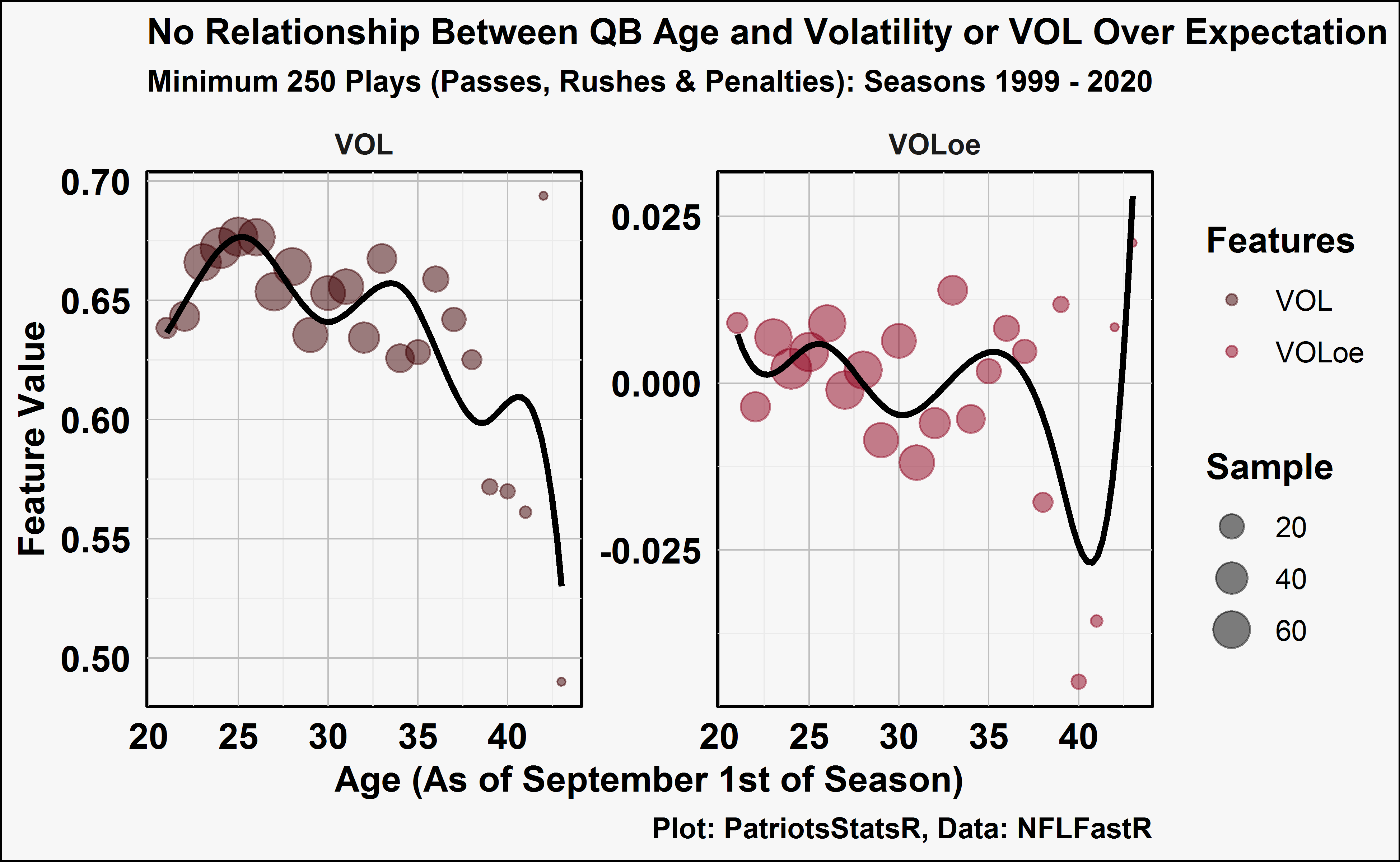
There doesn’t appear to be very much of a relationship. This is also a difficult question to answer because of survivorship bias. Good QB’s play longer, good QB’s also tend to have low volatility. Thus, volatile QB’s tend to be average to below average QB’s and don’t play as long.
Wrapping Up
This post demonstrated that on a macro scale, good QB’s have low volatility while middle of the pack QB’s tend to have the highest level of volatility. Raw volatility could be helpful for deciding between backup QB’s with similar EPA/Play (prefer the volatile bad QB due to the chance of a good game). Volatility over expected (VOLoe) can be used to detect high level EPA/Play seasons that also have a high VOLoe (possible indication of future regression).