Roll the clocks back to 2009. Tom Brady is back from tearing his ACL and MCL, Brett Favre is a Viking, and the Colts and Saints are a combined 26-0 by week 13. Nothing was quite as beautiful as what Darrelle Revis was doing for the New York Jets. Week after week, Revis would eliminate the opponent’s best receiver.
Measuring this dominance is hard however. Can we do better than just adding up the EPA from his swats and tackles, or just summarizing the defense as a whole? Instead of that, what if we ranked every team’s wide receivers and compared how each defense did against the opponent’s number one playmaker?
Data & transformations
First we need to load in the data, and to do that we follow Thomas Mock’s great guide on using Arrow to speed up the process.
library(arrow)
library(tidyverse)
library(ggrepel)
library(nflfastR)
library(ggpmisc)
options(mc.cores = parallel::detectCores())

set.seed(2009)

dir.create("nflfastr")

get_data <- function(year){
  dir.create(file.path("nflfastr", year))

  download.file(
    glue::glue("https://github.com/guga31bb/nflfastR-data/blob/master/data/play_by_play_{year}.parquet?raw=true"),
    file.path("nflfastr", year, "data.parquet"),
    mode = 'wb'
  )
}

walk(1999:2019, get_data)

ds <- open_dataset("nflfastr", partitioning = "year")
# We're grabbing everything since 1999 so I only have to do it once,
# but feel free to just do individual seasons
ds %>%
  select(
    desc,
    posteam,
    defteam,
    receiver,
    receiver_id,
    epa,
    cpoe,
    pass,
    qb_epa,
    air_yards,
    year,
    yards_gained,
    penalty
  ) %>%
  filter(year >= 1999, penalty == 0,!is.na(epa)) %>%
  collect() -> pbp
Next, we want to combine the play by play data with the roster data for receivers.
# Again, if you're just doing an individual season you can change this
nflfastR::fast_scraper_roster(1999:2020) -> roster

pbp %>%
  select(
    desc,
    posteam,
    defteam,
    receiver,
    receiver_id,
    epa,
    cpoe,
    pass,
    qb_epa,
    air_yards,
    year,
    yards_gained
  ) %>%
  filter(!is.na(receiver_id)) -> pbp2

pbp2 %>%
  left_join(roster, by = c("receiver_id" = "gsis_id")) -> pbp3
Now that we have the play by play merged with the roster data, we can go ahead and start transforming the data. We need to rank an offense’s wide receivers, and there are many ways to do so. For now, we’ll use targeted air yards, but we can change this decision later.
pbp3 %>%
  # we keep only the wide receivers, no tight ends or running backs
  filter(position == "WR") %>%
  group_by(receiver_id, year) %>%
  # we sum up all the receivers air yards when targeted
  mutate(targeted_air_yards = sum(air_yards)) %>%
  ungroup() %>%
  # distinct allows us to keep only one row per player
  distinct(receiver_id, year, .keep_all = T) %>%
  # we want to rank receivers by team, not overall, so we group by offense
  group_by(posteam, year) %>%
  # since we want to rank the receivers, arrange allows us to order them by some
  # criterion
  arrange(-targeted_air_yards) %>%
  # this index is now the within-team rank of each wide receiver that year
  mutate(index = row_number()) %>%
  ungroup() %>%
  select(receiver_id, targeted_air_yards, index, year) -> pbp4
Now that we have every receivers rank, we’ll add that back to the play by play data and remove any plays that didn’t have a receiver targeted.
At this point, I think the best way to graph this would be to compare how a defense does against WR 1, and against all other wide receivers. To do this, we’ll create a binary variable that says whether or not a receiver was number one. Uncreatively, I called this the smittywerbenjagermenjensen index, but you can rename it whatever you like.
pbp6 %>%
  mutate(smittywerbenjagermenjensen = if_else(index == 1, 1,0)) -> pbp7
Almost done. We’re going to group by the new smittywerbenjagermenjensen index and by defense and calculate the average EPA given up to WR 1 vs all others. Like ranking the receivers, there are lots of ways to skin a cat: possible options include using qb_epa instead, or CPOE, or summing any of the above instead of averaging them. All will give a slightly different answer.
pbp7 %>%
  group_by(defteam, smittywerbenjagermenjensen, year) %>%
  summarise(epa = mean(epa)) %>%
  ungroup() -> pbp8

# I could live to be 100 and never learn how to pivot correctly on the first try

pbp8 %>%
  pivot_wider(names_from = smittywerbenjagermenjensen,
              values_from =  epa,
              names_prefix = "wr_") -> pbp9

# We'll add the team colors so the graph looks nice

pbp9 %>%
  left_join(teams_colors_logos, by = c('defteam' = 'team_abbr')) -> pbp10

pbp10 %>%
  filter(year == 2009) -> pbp11
The plot (thickens)
Is it done? Yes! Now we can plot it and see which defenses could shutdown each opponent’s best receiver.
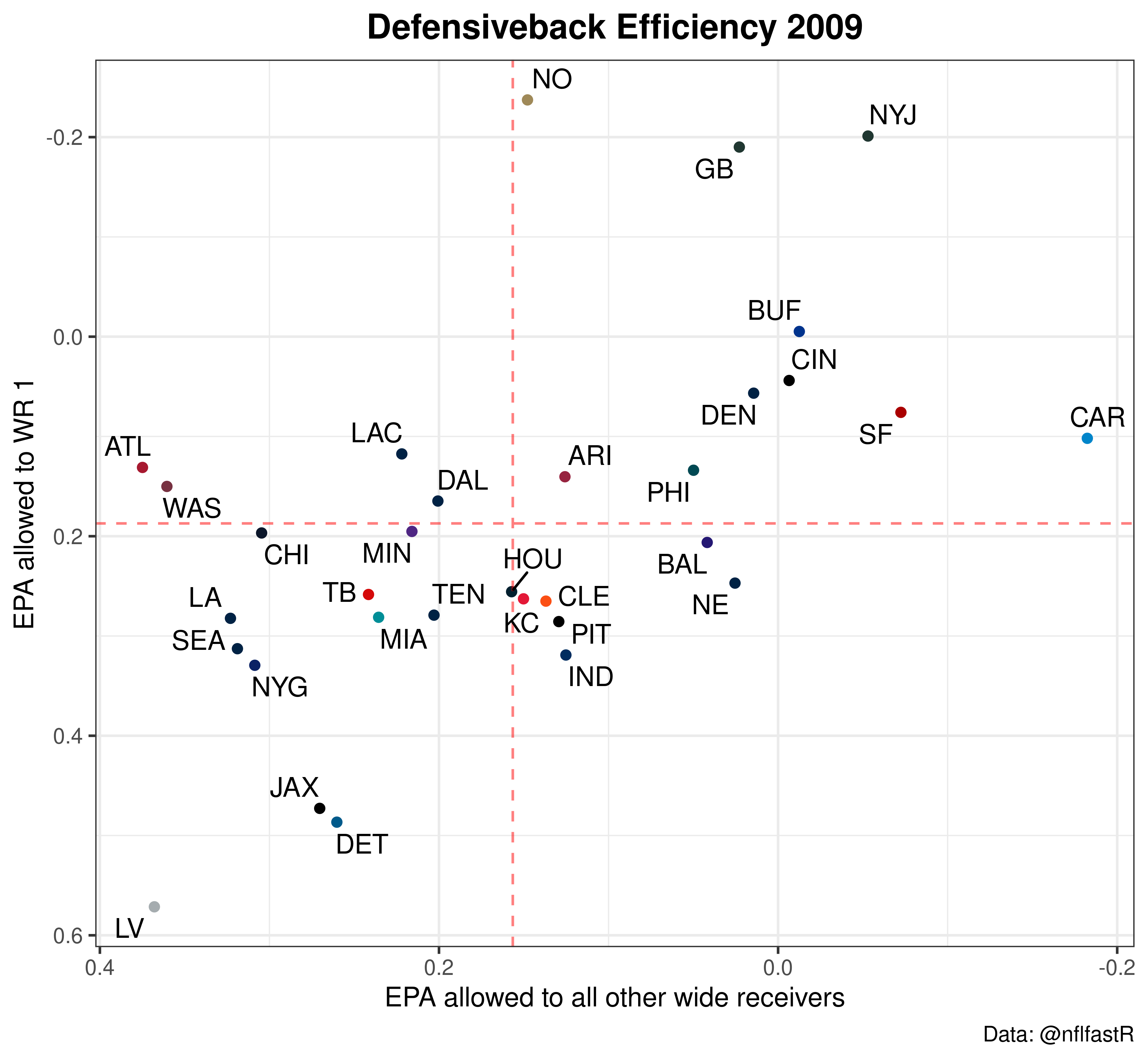
Wow! At a glance we can see that there are three teams that really shutdown the opponent’s best wide receiver. If you think back to ’09, even though Revis founded his island that year and solidified himself as the best cover corner in the league, it was Charles Woodson of the Packers who won defensive player of the year. In a very strange twist of fate however, the best performance was from New Orleans.
The coolest part about this, for me at least, is that we could recover all of these narratives from the data. Without measuring any cornerbacks directly, we can get a measurement that passes the eye test rather convincingly.
Of course, this measure is flawed in that we still can’t directly measure a player’s contribution. For example, the corners in New Orleans almost always had Darren Sharper over top to help him, and there’s no guarantee that they were actually covering WR 1 every play. For a player like Revis, you could argue that because he could eliminate the opponent’s WR 1 the rest of the defense could roll towards the other receivers and play them better, which is why the Jets are so much more rightward on the graph than the Saints.
Coda
We could argue endlessly about the best cover corners and seasons in NFL history, but as a coherence check I think we should take a look at how this new metric ranks every defense since 1999. To paraphrase Ben Baldwin, a coherence check for these models is “Do we find that Stephon Gilmore is in the top 5?”
With that in mind, let’s check out what the model thinks the best coverage season is. The code is mostly identical to the first section, but I put comments throughout the code to explain any changes. The biggest change is that we can’t use targeted air yards, since those don’t go far enough back, so I’ve elected to use total yards. Again, total EPA would be just as legitimate, as would targets or receptions. I invite you to play around with it.
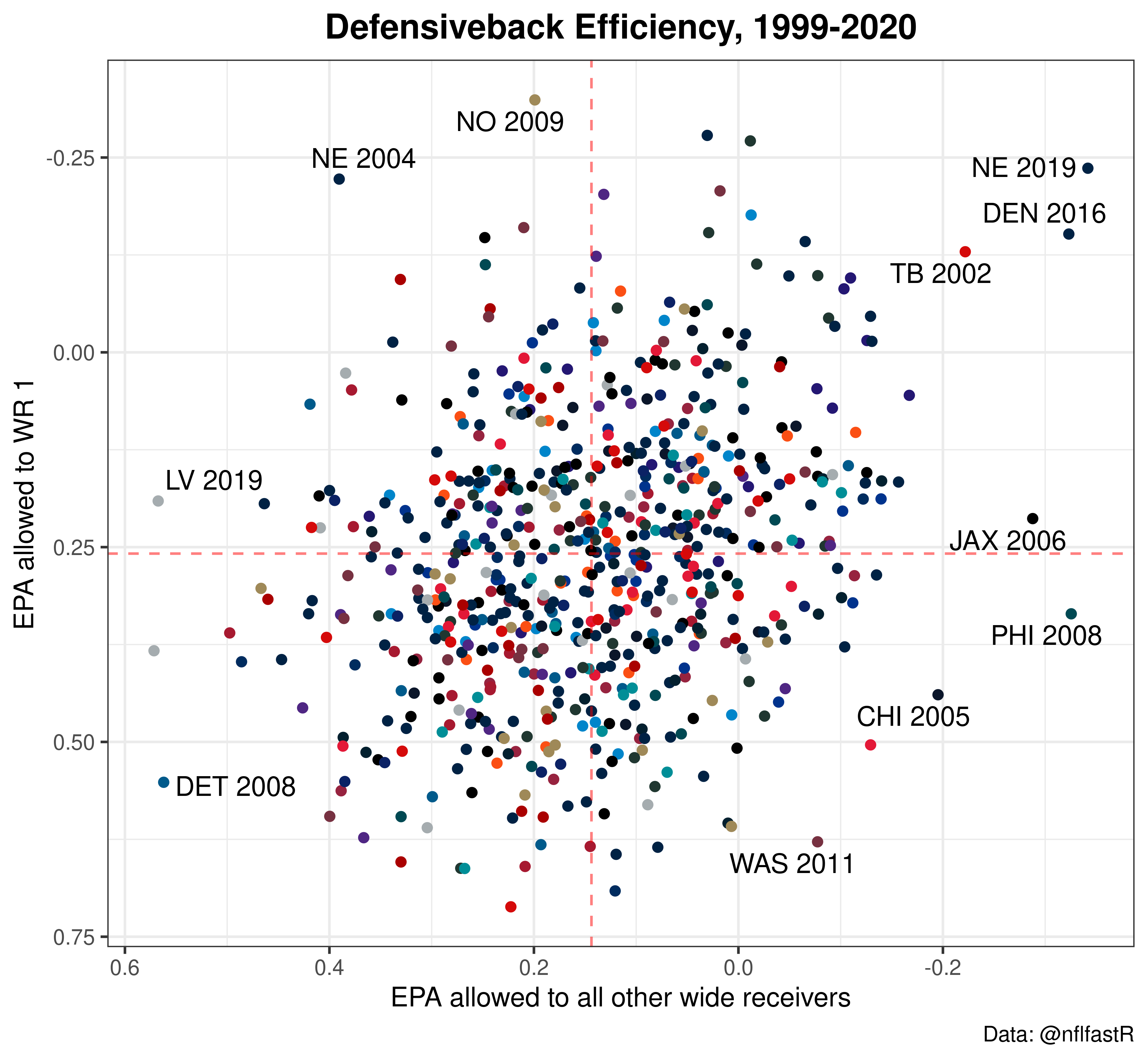
Sure enough, Stephon Gilmore’s 2019 season is in the top right, and ranks #4 since 1999. Surprisingly, that 2009 season by the Saints ranks as the best of the millennium. Just as surprising is that the Legion of Boom is nowhere in sight.
For the astute viewer, you may notice that the coverage score against WR 1 and against all other WRs is correlated. This could lend credibility to the theory that a shutdown corner allows the defense to divert resources elsewhere, or it could just be that good coordinators get better performances from all corners.
This is by no means the be-all end-all of cornerback rankings. I’d love to see this extended to account for the quality of receivers faced and for different eras. A version looking at all receivers, including TEs and RBs, may be even more enlightening. Finally, like the team tiers, average EPA allowed to WR 1 is worth a different amount than the average EPA allowed to all other receivers, and it would be great to sort these defenses into tiers, as well as do a stability analysis to see if any of these measures are more stable than regular defense.