The winners of the 2019 and 2020 Big Data Bowls each used Convolutional Neural Networks (CNNs) in their winning entries. This approach essentially treats player tracking data as an image recognition problem and then applies well established computer vision techniques. In this post, we’ll dive into what that actually entails.
Computer Vision Background
If you don’t know anything about computer vision and would like to learn, I personally found this University of Michigan course taught by Justin Johnson incredibly helpful. Here is a link to the lecture videos, here is the syllabus and PDFs of the lecture slides, and see the first link for the homework assignments (which are in PyTorch; i.e. Python). To understand what’s happening in the course, some familiarity with how to manipulate matrices is very useful, especially if you try to tackle the homework assignments.
An aside: If you haven’t done anything like this before, a lot of this post will not make a lot of sense. What we will do here is a lot different than learning how to use, for example, xgboost, for a couple reasons. First, we’re departing from the comfort of the “rectangular” data structure where each row is an observation and each column is a feature. In computer vision problems, there are typically (at least) four dimensions: one for each observation, another for each feature dimension (e.g. 3 for a typical red-green-blue image), one for the height of the image, and one for the width. And second, there’s a lot more housekeeping that needs to be done in the code: keeping track of batches, telling it to compute gradients and update weights, and some other stuff along these lines. If none of this makes sense, that’s okay! If you watch the lectures linked above (and even more so, try the homeworks) and come back to this, everything will make a lot more sense.
It’s no accident that the course linked above uses PyTorch. Python is the dominant language for computer vision. However, there is recent good news for R users: torch in R has been developed and contains basically all of the same things as the Python version, which means that if you’re already comfortable with R, you don’t need to learn a whole new language just to do computer vision stuff (plus trying to clean and manipulate data in pandas is the worst).
The Goals for this Post
- Yes: demonstrate how to use torch in R and what this looks like when using NFL player tracking data
- No: create the most accurate model possible
Since this is Open Source Football, I’m only going to use things that others can access to: i.e., the tracking data and coverage labels provided through Big Data Bowl 2021. In particular, this means that this post will only be working with coverage labels from week 1 of the 2018 season since that is what was provided to contestants. If you want to replicate this post, you’ll need to get the player tracking data here and the coverage labels here. If one had access to a full season of coverage labels, hypothetically speaking, one could train a much better model. In addition, since this designed to be an introductory post, I’m only going to use one frame per play, which limits the accuracy a bit.
Let’s get to it!
Load the Data
I’m going to mostly skip over the data cleaning stuff this since it isn’t the focus of the post, plus I wrote a package that gets all of the annoying data prep out of the way. If you’re interested, you can check out the code in the package, and maybe by the time you’re reading this I’ll have even documented the functions (ha ha). The function below takes week 1 of the 2021 Big Data Bowl, makes all plays go from left to right, adds some columns like the extent to which each defender’s orientation points him at the quarterback, and gets some information about each play (e.g. whether each player is on offense or defense and the location of the line of scrimmage).
library(tidyverse)
library(torch)
library(patchwork)
library(gt)

df <- ngscleanR::prepare_bdb_week(
  week = 1,
  dir = "../../../nfl-big-data-bowl-2021/input",
  # any throw that happens before 1.5 seconds after snap is thrown away
  trim_frame = 25,
  # all frames coming more than 1 second after pass released are thrown away
  frames_after_throw = 10,
  # let's keep this frame for fun (1.8 seconds after snap)
  keep_frames = c(31)
)
Now let’s get the labels from 2018 week 1 with thanks to Telemetry.
labels <- readr::read_csv("../../../nfl-big-data-bowl-2021/input/coverages_week1.csv") %>%
  mutate(
    play = paste0(gameId, "_", playId)
  ) %>%
  filter(!is.na(coverage)) %>%
  select(play, coverage)

df <- df %>%
  inner_join(labels, by = "play")

# check labels
labels %>%
  group_by(coverage) %>%
  summarize(n = n()) %>%
  ngscleanR:::make_table()
| coverage | n |
|---|---|
| Cover 0 Man | 13 |
| Cover 1 Man | 296 |
| Cover 2 Man | 32 |
| Cover 2 Zone | 113 |
| Cover 3 Zone | 352 |
| Cover 4 Zone | 152 |
| Cover 6 Zone | 69 |
| Prevent Zone | 1 |
Data Wrangling / Create Tensors
For reference, here’s what the location and orientation columns in Big Data Bowl mean:
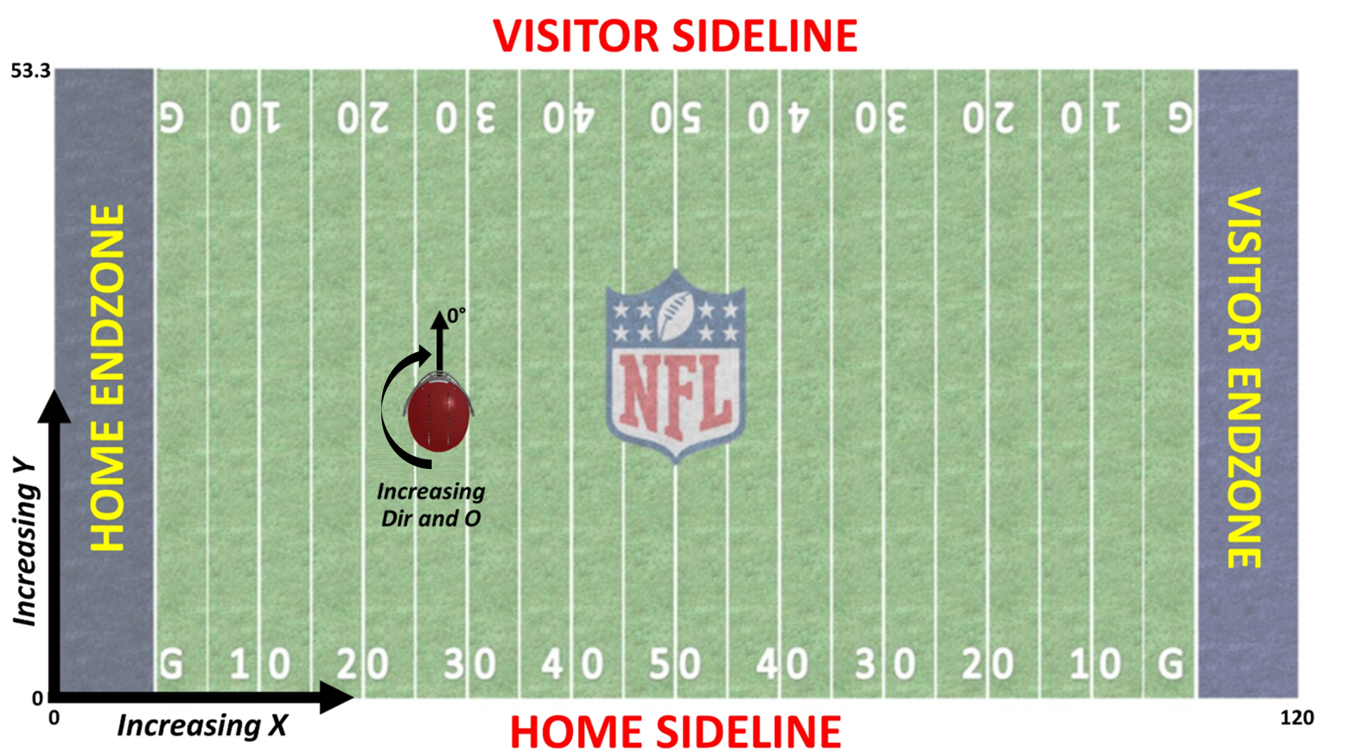
And we want to create something along the lines of The Zoo’s solution but modified to predict coverages rather than the result of a rushing play. In particular, this section is creating the blue part of this on the left:
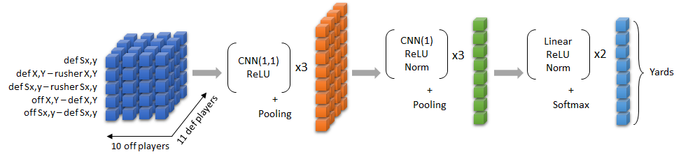
In The Zoo’s entry, they had 10 feature dimensions ((a) defender position, (b) defender position relative to the rusher, (c) defender speed relative to the rusher, (d) defender position relative to offensive player, and (e) defender speed relative to offensive player, all in both the X and Y directions). But their problem was different because they were trying to predict the results of a run play. For coverage classification, things like speed relative to the rusher don’t make sense. There is no rusher! For this post, I’ve settled on 13 features, but haven’t done a lot of playing around with other features so there might be better ways to do this. Here are the features we’ll create:
- 1: Distance from line of scrimmage (this serves as X location)
- 2: Y location
- 3 and 4: Speed in X and Y directions
- 5 and 6: Acceleration in X and Y directions
- 7: Orientation towards quarterback (measured 0 to 1, with 0 meaning facing directly at QB, 1 directly away)
- 8 and 9: X and Y distance from each offensive player
- 10 and 11: X and Y speed relative to each offensive player
- 12 and 13: X and Y acceleration relative to each offensive player
Because the maximum number of non-QB offensive players provided in Big Data Bowl is 5 and defensive players 11, we will be creating a tensor – basically a higher-dimensional matrix used by torch – of size (number of plays) x (13) x (11) x (5), with 13 being the number of features (listed above), 11 the number of defenders, and 5 offensive players. Each of the 13 features will have a 11 x 5 matrix that gives a value for each defensive player relative to each offensive player. For example, the entry (1, 13, 1, 1) would pull out the difference in acceleration in the Y direction (i.e., the 13th feature) between the 1st defensive player and 1st offensive player on the 1st play, and the entry (1, 13, ..) would give an 11 by 5 matrix of the relative speed of each possible combination of defensive player and offensive player. If you’re wondering how to choose who the “1st defensive player” is, the beauty of The Zoo’s solution is that you can put the players in any order and the model will treat them the same; i.e., the order doesn’t matter.
Since we need to get a data frame of defenders relative to offensive players, let’s do that using the pre-cleaned data by joining an offense dataframe to a defense dataframe by play, which joins each offensive player to each possible defensive player:
offense_df <- df %>%
  filter(defense == 0) %>%
  select(play, frame_id, o_x = x, o_y = y, o_s_x = s_x, o_s_y = s_y, o_a_x = a_x, o_a_y = a_y)

defense_df <- df %>%
  filter(defense == 1) %>%
  select(play, frame_id, nfl_id, x, y, s_x, s_y, a_x, a_y, o_to_qb, dist_from_los)

rel_df <- defense_df %>%
  # since there are duplicates at each play & frame this creates 1 entry per offense-defense player combination
  left_join(offense_df, by = c("play", "frame_id")) %>%
  mutate(diff_x = o_x - x, diff_y = o_y - y, diff_s_x = o_s_x - s_x, diff_s_y = o_s_y - s_y, diff_a_x = o_a_x - a_x, diff_a_y = o_a_y - a_y) %>%
  select(play, frame_id, nfl_id, dist_from_los, y, s_x, s_y, a_x, a_y, o_to_qb, starts_with("diff_"))

rel_df %>%
  select(nfl_id, dist_from_los, y, diff_x, diff_y) %>%
  head(10) %>%
  ngscleanR:::make_table()
| nfl_id | dist_from_los | y | diff_x | diff_y |
|---|---|---|---|---|
| 2539334 | 4.03 | 15.46333 | -0.37 | -1.47 |
| 2539334 | 4.03 | 15.46333 | -0.88 | 16.43 |
| 2539334 | 4.03 | 15.46333 | -8.70 | 15.81 |
| 2539334 | 4.03 | 15.46333 | 0.93 | 22.14 |
| 2539334 | 4.03 | 15.46333 | -6.18 | 6.53 |
| 2539653 | 5.28 | 38.06333 | -1.62 | -24.07 |
| 2539653 | 5.28 | 38.06333 | -2.13 | -6.17 |
| 2539653 | 5.28 | 38.06333 | -9.95 | -6.79 |
| 2539653 | 5.28 | 38.06333 | -0.32 | -0.46 |
| 2539653 | 5.28 | 38.06333 | -7.43 | -16.07 |
The first 5 entries here represent the first defensive player matched to each of the 5 offensive players. Note that a lot of the columns are constant for the first 5 rows because each row represents a defense-offense match and many entries do not depend on the offensive player. For example, the defender’s distance from the line of scrimmage is the same for each matched offensive player (in The Zoo’s entry, this is what they mean by some features being “constant across ‘off’ dimension of the tensor”).
For some housekeeping, let’s save a master list of plays to refer to later.
play_indices <- df %>%
  select(play, frame_id, play, week, coverage) %>%
  unique() %>%
  # get play index for 1 : n_plays
  mutate(
    i = as.integer(as.factor(play))
  ) %>%
  # get time step indices
  # this is useless for this post bc we're only using one frame
  # but useful when extending to more frames
  group_by(play) %>%
  mutate(f = 1:n()) %>%
  ungroup()

n_frames <- n_distinct(play_indices$f)
n_plays <- n_distinct(play_indices$i)
n_class <- n_distinct(play_indices$coverage)

def_only_features <- 7
off_def_features <- 6
n_features <- def_only_features + off_def_features

play_indices %>%
  head(10) %>%
  ngscleanR:::make_table()
| play | frame_id | week | coverage | i | f |
|---|---|---|---|---|---|
| 2018090600_1037 | 31 | 1 | Cover 2 Man | 1 | 1 |
| 2018090600_1061 | 31 | 1 | Cover 1 Man | 2 | 1 |
| 2018090600_1085 | 31 | 1 | Cover 3 Zone | 3 | 1 |
| 2018090600_1202 | 31 | 1 | Cover 3 Zone | 4 | 1 |
| 2018090600_1226 | 31 | 1 | Cover 1 Man | 5 | 1 |
| 2018090600_1295 | 31 | 1 | Cover 1 Man | 6 | 1 |
| 2018090600_1344 | 31 | 1 | Cover 4 Zone | 7 | 1 |
| 2018090600_1423 | 31 | 1 | Cover 3 Zone | 8 | 1 |
| 2018090600_146 | 31 | 1 | Cover 3 Zone | 9 | 1 |
| 2018090600_1473 | 31 | 1 | Cover 3 Zone | 10 | 1 |
Now we’re ready to start making our tensor, which is what torch knows how to deal with. Note that I’m throwing in an extra dimension for number of frames on each play, which is useless in this case (1 frame per play) but makes it easier to extend to using multiple frames in a given play (the real reason I’m doing this is that my existing code uses more frames and it’s easier to not re-write this part of it).
data_tensor <- torch_empty(n_plays, n_frames, n_features, 11, 5)
dim(data_tensor)
#> [1] 1018 1 13 11 5Here is the function that will help us populate our tensor, explained below.
fill_row <- function(row) {

  # indices for putting in tensor
  i <- row$i # row
  f <- row$f # frame

  # play info for extracting from df
  playid <- row$play
  frameid <- row$frame_id

  play_df <- rel_df %>%
    filter(play == playid, frame_id == frameid) %>%
    select(-play, -frame_id)

  # how many defense and offense players are there on this play?
  defenders <- n_distinct(play_df$nfl_id)
  n_offense <- nrow(play_df) / defenders

  # get rid of player ID since it's not in the model
  play_df <- play_df %>% select(-nfl_id)

  # where the magic happens
  # explanation of this part below!
  data_tensor[i, f, , 1:defenders, 1:n_offense] <-
    torch_tensor(t(play_df))$view(c(-1, defenders, n_offense))
}
Digression into Wrangling This Data
If you haven’t worked with higher-dimensional data before, it can be kind of hard to wrap your head around. Let’s illustrate what is happening in the function above using the first play as an example. Here is what the raw data look like when running this function on the first play (showing the first 10 rows):
row <- play_indices %>% dplyr::slice(1)

i <- row$i
f <- row$f

playid <- row$play
frameid <- row$frame_id

play_df <- rel_df %>%
  filter(play == playid, frame_id == frameid) %>%
  select(-play, -frame_id)

defenders <- n_distinct(play_df$nfl_id)
n_offense <- nrow(play_df) / defenders

play_df <- play_df %>% select(-nfl_id)

defenders
#> [1] 7dim(play_df)
#> [1] 35 13
play_df %>%
  head(10) %>%
  ngscleanR:::make_table()
| dist_from_los | y | s_x | s_y | a_x | a_y | o_to_qb | diff_x | diff_y | diff_s_x | diff_s_y | diff_a_x | diff_a_y |
|---|---|---|---|---|---|---|---|---|---|---|---|---|
| 4.03 | 15.46333 | 5.270580 | -3.648162 | 2.442063 | -1.6903340 | 0.9869417 | -0.37 | -1.47 | 0.6550943 | -0.02161781 | 0.2784763 | 0.005499684 |
| 4.03 | 15.46333 | 5.270580 | -3.648162 | 2.442063 | -1.6903340 | 0.9869417 | -0.88 | 16.43 | -0.4223971 | -0.15193297 | -0.5216787 | 0.185101602 |
| 4.03 | 15.46333 | 5.270580 | -3.648162 | 2.442063 | -1.6903340 | 0.9869417 | -8.70 | 15.81 | -5.7954932 | 2.80877747 | -3.7516945 | -0.403887787 |
| 4.03 | 15.46333 | 5.270580 | -3.648162 | 2.442063 | -1.6903340 | 0.9869417 | 0.93 | 22.14 | 0.2337943 | 1.72702611 | -0.6765088 | 1.074120621 |
| 4.03 | 15.46333 | 5.270580 | -3.648162 | 2.442063 | -1.6903340 | 0.9869417 | -6.18 | 6.53 | -4.6102605 | -1.42907927 | -1.9377953 | -2.187012303 |
| 5.28 | 38.06333 | 4.597714 | -1.605593 | 2.039232 | -0.7121318 | 0.2054857 | -1.62 | -24.07 | 1.3279608 | -2.06418628 | 0.6813069 | -0.972702512 |
| 5.28 | 38.06333 | 4.597714 | -1.605593 | 2.039232 | -0.7121318 | 0.2054857 | -2.13 | -6.17 | 0.2504695 | -2.19450144 | -0.1188481 | -0.793100594 |
| 5.28 | 38.06333 | 4.597714 | -1.605593 | 2.039232 | -0.7121318 | 0.2054857 | -9.95 | -6.79 | -5.1226266 | 0.76620901 | -3.3488640 | -1.382089984 |
| 5.28 | 38.06333 | 4.597714 | -1.605593 | 2.039232 | -0.7121318 | 0.2054857 | -0.32 | -0.46 | 0.9066608 | -0.31554235 | -0.2736782 | 0.095918425 |
| 5.28 | 38.06333 | 4.597714 | -1.605593 | 2.039232 | -0.7121318 | 0.2054857 | -7.43 | -16.07 | -3.9373939 | -3.47164774 | -1.5349648 | -3.165214499 |
We need to have this thing be 13 x 7 x 5 (7 defenders and 5 offensive players on this play), but right now it is (5 x 7) x 13 with each group of 5 rows a set of rows for each defensive player, and the features going across as columns rather than as rows like we need for the tensor shape.
The first step is to transpose (showing first 8 columns so it’s not huge):
# showing first 8 columns so this isn't huge
t(play_df)[, 1:8]
#>                       [,1]       [,2]       [,3]       [,4]
#> dist_from_los  4.030000000  4.0300000  4.0300000  4.0300000
#> y             15.463333333 15.4633333 15.4633333 15.4633333
#> s_x            5.270580108  5.2705801  5.2705801  5.2705801
#> s_y           -3.648161911 -3.6481619 -3.6481619 -3.6481619
#> a_x            2.442062858  2.4420629  2.4420629  2.4420629
#> a_y           -1.690333990 -1.6903340 -1.6903340 -1.6903340
#> o_to_qb        0.986941709  0.9869417  0.9869417  0.9869417
#> diff_x        -0.370000000 -0.8800000 -8.7000000  0.9300000
#> diff_y        -1.470000000 16.4300000 15.8100000 22.1400000
#> diff_s_x       0.655094267 -0.4223971 -5.7954932  0.2337943
#> diff_s_y      -0.021617811 -0.1519330  2.8087775  1.7270261
#> diff_a_x       0.278476310 -0.5216787 -3.7516945 -0.6765088
#> diff_a_y       0.005499684  0.1851016 -0.4038878  1.0741206
#>                     [,5]        [,6]       [,7]       [,8]
#> dist_from_los  4.0300000   5.2800000  5.2800000  5.2800000
#> y             15.4633333  38.0633333 38.0633333 38.0633333
#> s_x            5.2705801   4.5977135  4.5977135  4.5977135
#> s_y           -3.6481619  -1.6055934 -1.6055934 -1.6055934
#> a_x            2.4420629   2.0392323  2.0392323  2.0392323
#> a_y           -1.6903340  -0.7121318 -0.7121318 -0.7121318
#> o_to_qb        0.9869417   0.2054857  0.2054857  0.2054857
#> diff_x        -6.1800000  -1.6200000 -2.1300000 -9.9500000
#> diff_y         6.5300000 -24.0700000 -6.1700000 -6.7900000
#> diff_s_x      -4.6102605   1.3279608  0.2504695 -5.1226266
#> diff_s_y      -1.4290793  -2.0641863 -2.1945014  0.7662090
#> diff_a_x      -1.9377953   0.6813069 -0.1188481 -3.3488640
#> diff_a_y -2.1870123 -0.9727025 -0.7931006 -1.3820900#> [1] 13 35Now we’re closer, with the data shaped 13 x (5 X 7). That is, there are now 13 rows with each row a feature like we want, but columns 1-5 represent the first defender, 6-10 the second, etc (I’ve only shown the first 10 columns above so the output isn’t huge on the page). We need to take each of these and split up the defenders into different dimensions so that we end up with 13 sets of 7 x 5 matrices.
The below is the complete line for getting to the right shape (if you find this part hard to follow, don’t feel like it’s supposed to be easy; this took me a lot of trial and error while working with little toy examples).
torch_tensor(t(play_df))$view(c(-1, defenders, n_offense))
#> torch_tensor
#> (1,.,.) =
#>    4.0300   4.0300   4.0300   4.0300   4.0300
#>    5.2800   5.2800   5.2800   5.2800   5.2800
#>   19.3800  19.3800  19.3800  19.3800  19.3800
#>   -4.5100  -4.5100  -4.5100  -4.5100  -4.5100
#>    3.3900   3.3900   3.3900   3.3900   3.3900
#>   14.2700  14.2700  14.2700  14.2700  14.2700
#>    1.7400   1.7400   1.7400   1.7400   1.7400
#>
#> (2,.,.) =
#>   15.4633  15.4633  15.4633  15.4633  15.4633
#>   38.0633  38.0633  38.0633  38.0633  38.0633
#>   25.5533  25.5533  25.5533  25.5533  25.5533
#>   30.8233  30.8233  30.8233  30.8233  30.8233
#>   32.8033  32.8033  32.8033  32.8033  32.8033
#>   31.6433  31.6433  31.6433  31.6433  31.6433
#>   23.6133  23.6133  23.6133  23.6133  23.6133
#>
#> (3,.,.) =
#>   5.2706  5.2706  5.2706  5.2706  5.2706
#>   4.5977  4.5977  4.5977  4.5977  4.5977
#>   2.5835  2.5835  2.5835  2.5835  2.5835
#>  -3.1190 -3.1190 -3.1190 -3.1190 -3.1190
#>   4.2293  4.2293  4.2293  4.2293  4.2293
#>   5.3371  5.3371  5.3371  5.3371  5.3371
#>   0.1803  0.1803  0.1803  0.1803  0.1803
#>
#> (4,.,.) =
#>  -3.6482 -3.6482 -3.6482 -3.6482 -3.6482
#>  -1.6056 -1.6056 -1.6056 -1.6056 -1.6056
#> ... [the output was truncated (use n=-1 to disable)]
#> [ CPUFloatType{13,7,5} ]
Hooray! It looks like it should. We have a 13x7x5 tensor with each of the 13 feature dimensions carrying a 7x5 matrix that matches each of the 7 defensive players to each of the 5 offensive players. Note that we’re starting to use torch stuff for the first time, where view is a function that reshapes tensors that will be familiar to anyone who has used PyTorch.
Hopefully this sheds some light on the above function. Now let’s use it.
Fill in the Tensors
Digression over and back to work. This iterates over every play to fill in the tensor for each play.
Let’s make sure it worked:
data_tensor[1, ..]
#> torch_tensor
#> (1,1,.,.) =
#>    4.0300   4.0300   4.0300   4.0300   4.0300
#>    5.2800   5.2800   5.2800   5.2800   5.2800
#>   19.3800  19.3800  19.3800  19.3800  19.3800
#>   -4.5100  -4.5100  -4.5100  -4.5100  -4.5100
#>    3.3900   3.3900   3.3900   3.3900   3.3900
#>   14.2700  14.2700  14.2700  14.2700  14.2700
#>    1.7400   1.7400   1.7400   1.7400   1.7400
#>    0.0000   0.0000   0.0000   0.0000   0.0000
#>    0.0000   0.0000   0.0000   0.0000   0.0000
#>    0.0000   0.0000   0.0000   0.0000   0.0000
#>    0.0000   0.0000   0.0000   0.0000   0.0000
#>
#> (1,2,.,.) =
#>   15.4633  15.4633  15.4633  15.4633  15.4633
#>   38.0633  38.0633  38.0633  38.0633  38.0633
#>   25.5533  25.5533  25.5533  25.5533  25.5533
#>   30.8233  30.8233  30.8233  30.8233  30.8233
#>   32.8033  32.8033  32.8033  32.8033  32.8033
#>   31.6433  31.6433  31.6433  31.6433  31.6433
#>   23.6133  23.6133  23.6133  23.6133  23.6133
#>    0.0000   0.0000   0.0000   0.0000   0.0000
#>    0.0000   0.0000   0.0000   0.0000   0.0000
#>    0.0000   0.0000   0.0000   0.0000   0.0000
#>    0.0000   0.0000   0.0000   0.0000   0.0000
#>
#> (1,3,.,.) =
#>   5.2706  5.2706  5.2706  5.2706  5.2706
#>   4.5977  4.5977  4.5977  4.5977  4.5977
#>   2.5835  2.5835  2.5835  2.5835  2.5835
#> ... [the output was truncated (use n=-1 to disable)]
#> [ CPUFloatType{1,13,11,5} ]
This shows that the first play has been filled in. The extra zeroes in the final rows are because we initialized a tensor of zeroes for 11 defenders, but not all defenders are provided on every play, so a lot of plays will have zeroes like this. I think about it like a bunch of players standing in the corner of the field together not impacting the play since that’s basically what the computer sees (I tried sticking all the “missing” players on the line of scrimmage standing there looking at each other, but it didn’t seem to make much of a difference).
Now let’s fill in the coverage labels. Note that the torch_long() part is required for labels and the labels have to be integers starting from 1.
label_tensor <- torch_zeros(n_plays, dtype = torch_long())

label_tensor[1:n_plays] <- play_indices %>%
  mutate(coverage = as.factor(coverage) %>% as.integer()) %>%
  pull(coverage)
Finally, I need to get rid of the time dimension since I’m not using it here (torch_squeeze gets rid of any singleton dimensions).
data_tensor <- torch_squeeze(data_tensor)
dim(data_tensor)
#> [1] 1018 13 11 5dim(label_tensor)
#> [1] 1018Now we have about 1,000 plays from week 1 shaped in the way we want.
Split the data
Let’s hold out 200 plays for testing and split the remaining sample into 5 sets of 80% training and 20% validation splits.
test_size <- 200
set.seed(2013) # gohawks

# hold out
test_id <- sample(1:n_plays, size = test_size)
test_data <- data_tensor[test_id, ..]
test_label <- label_tensor[test_id]

# full training set
train_id <- setdiff(1:n_plays, test_id)
train_data <- data_tensor[train_id, ..]
train_label <- label_tensor[train_id]

# helper thing that is just 1, ..., length train data
all_train_idx <- 1:dim(train_data)[1]

# create folds from the train indices
# stratified by label
folds <- splitTools::create_folds(
  y = as.integer(train_label),
  k = 5,
  type = "stratified",
  invert = TRUE
)

dim(train_data)
#> [1] 818 13 11 5dim(train_label)
#> [1] 818str(folds)
#> List of 5
#>  $ Fold1: int [1:164] 2 6 10 14 17 24 29 43 53 66 ...
#>  $ Fold2: int [1:163] 5 11 15 18 21 23 34 35 44 48 ...
#>  $ Fold3: int [1:162] 1 7 8 12 13 16 20 31 40 41 ...
#>  $ Fold4: int [1:164] 4 9 19 26 28 32 33 37 42 52 ...
#>  $ Fold5: int [1:165] 3 22 25 27 30 36 38 39 45 46 ...
The folds object created above is a list of 5 where each item in the list is the set of validation indices for a given fold.
Data Augmentation
From The Zoo’s entry:
What worked really well for us is to add augmentation and TTA for Y coordinates. We assume that in a mirrored world the runs would have had the same outcomes. For training, we apply 50% augmentation to flip the Y coordinates (and all respective relative features emerging from it)
So we need a function that flips any features related to Y vertically. That is below.
augment_data <- function(df,
                         # stuff that will be multiplied by -1 (eg Sy)
                         flip_indices = c(4, 6, 9, 11, 13),
                         # raw y location
                         subtract_indices = c(2)) {


  # indices of the elements that need to be flipped
  t <- torch_ones_like(df)
  t[, flip_indices, , ] <- -1

  # first fix: multiply by -1 where needed (stuff like speed in Y direction)
  flipped <- df * t

  # for flipping Y itself, need to do 160/3 - y
  t <- torch_zeros_like(df)
  t[, subtract_indices, , ] <- 160 / 3

  # second fix: flip around y
  flipped[, subtract_indices, , ] <- t[, subtract_indices, , ] - flipped[, subtract_indices, , ]

  return(flipped)
}
This will be used below during training (when augmenting the data by adding flipped data) and testing (when getting the prediction as an average of the flipped and non-flipped data).
Datasets and Dataloaders
Okay, so we have tensors, and now we need to turn them into something that can be used in training. For this, we need torch’s dataset(), which is way to easily fetch of observations at once. This is mostly copy and pasting from the below link and not that interesting.
Another possible workflow is to put all the data cleaning and preparation work done above into the dataset() function, which would probably make for a simpler predict stage when putting something like this into production, but I haven’t done this yet.
Now let’s stick our data in the dataset:
train_ds <- tracking_dataset(train_data, train_label)
Alright, so what did that actually do? Now we can access the .getitem() and .length() things created in the dataset() definition above, which would show the first item in the training dataset (if we ran train_ds$.getitem(1)), or the total length of the dataset (train_ds$.length()).
You might have thought we’re done now, but not quite. Now we need to send our dataset to a dataloader .
# Dataloaders
train_dl <- train_ds %>%
  dataloader(batch_size = 64, shuffle = TRUE)
The dataloaders allow for torch to access the data in batches, which as we’ll see below, is how the model is trained.
This shows how many batches we have:
train_dl$.length()
#> [1] 13And this shows one of the batches, and we can refer to the data and labels as x and y because of how we constructed the dataset above:
Both the data and labels have 64 rows as expected (the batch size).
The Model
This is a straight copy of The Zoo’s model so there’s not much to say here, but I will leave some comments to explain what is happening.
net <- nn_module(
  "Net",
  initialize = function() {
    self$conv_block_1 <- nn_sequential(
      nn_conv2d(
        # 1x1 convolution taking in 13 (n_features) channels and outputting 128
        # before: batch * 13 * 11 * 5
        # after: batch * 128 * 11 * 5
        in_channels = n_features,
        out_channels = 128,
        kernel_size = 1
      ),
      nn_relu(inplace = TRUE),
      nn_conv2d(
        in_channels = 128,
        out_channels = 160,
        kernel_size = 1
      ),
      nn_relu(inplace = TRUE),
      nn_conv2d(
        in_channels = 160,
        out_channels = 128,
        kernel_size = 1
      ),
      nn_relu(inplace = TRUE),
    )

    self$conv_block_2 <- nn_sequential(
      nn_batch_norm1d(128),
      nn_conv1d(
        in_channels = 128,
        out_channels = 160,
        kernel_size = 1
      ),
      nn_relu(inplace = TRUE),
      nn_batch_norm1d(160),
      nn_conv1d(
        in_channels = 160,
        out_channels = 96,
        kernel_size = 1
      ),
      nn_relu(inplace = TRUE),
      nn_batch_norm1d(96),
      nn_conv1d(
        in_channels = 96,
        out_channels = 96,
        kernel_size = 1
      ),
      nn_relu(inplace = TRUE),
      nn_batch_norm1d(96)
    )

    self$linear_block <- nn_sequential(
      nn_linear(96, 96),
      nn_relu(inplace = TRUE),
      nn_batch_norm1d(96),
      nn_linear(96, 256),
      nn_relu(inplace = TRUE),

      # note: breaks on current kaggle version
      nn_batch_norm1d(256),
      nn_layer_norm(256),
      nn_dropout(p = 0.3),

      # n_class is how many distinct labels there are
      nn_linear(256, n_class)
    )
  },
  forward = function(x) {

    # first conv layer
    # outputs batch * 128 * 11 * 5
    x <- self$conv_block_1(x)

    # first pool layer: average of mean and max pooling
    # the 5 is number of offensive players
    avg <- nn_avg_pool2d(kernel_size = c(1, 5))(x) %>%
      torch_squeeze(-1)
    max <- nn_max_pool2d(kernel_size = c(1, 5))(x) %>%
      torch_squeeze(-1)

    x <- 0.7 * avg + 0.3 * max

    # x is now batch * 128 * 11

    # second conv layer
    x <- self$conv_block_2(x)

    # second pool layer
    avg <- nn_avg_pool1d(kernel_size = 11)(x) %>%
      torch_squeeze(-1)
    max <- nn_max_pool1d(kernel_size = 11)(x) %>%
      torch_squeeze(-1)

    x <- 0.7 * avg + 0.3 * max

    # x is now batch * 96

    x <- self$linear_block(x)

    # x is now batch * # labels

    x
  }
)
Training with Cross Validation
We’ve done a lot of setup to get to this point, and now we can actually train a model!
I’m going to use what is known as k-fold validation (with k = 5 in this case). For each of the 5 folds, we estimate a separate model using 80% of the data as the training set and the remaining 20% as the validation set. This helps give a more realistic expectation of what to expect from final testing than using one fold, especially here since our data are so limited. Looking at the below, the accuracy among the 5 folds ranges from 73% - 82%, with an average of 78%.
At the predict stage to follow, we could either average over these 5 models (this is what I do) or re-train on the entire train set. Reading through the link above, it seems like the choice of which to do is not super obvious (and might not matter that much).
Here’s the big loop:
set.seed(2013)
torch_manual_seed(2013)

accuracies <- torch_zeros(length(folds))
best_epochs <- torch_zeros(length(folds))

epochs <- 50

# start iteration over folds
for (fold in 1:length(folds)) {
  cat(sprintf("\n------------- FOLD %d ---------", fold))

  model <- net()
  optimizer <- optim_adam(model$parameters, lr = 0.001)
  scheduler <- lr_step(optimizer, step_size = 1, 0.975)

  # extract train and validation sets
  val_i <- folds[[fold]]
  train_i <- all_train_idx[-val_i]

  .ds_train <- dataset_subset(train_ds, train_i)
  .ds_val <- dataset_subset(train_ds, val_i)

  .train_dl <- .ds_train %>%
    dataloader(batch_size = 64, shuffle = TRUE)
  .valid_dl <- .ds_val %>%
    dataloader(batch_size = 64, shuffle = TRUE)

  for (epoch in 1:epochs) {
    train_losses <- c()
    valid_losses <- c()
    valid_accuracies <- c()

    # train step: loop over batches
    model$train()
    for (b in enumerate(.train_dl)) {

      # augment first
      b_augmented <- augment_data(b$x)
      x <- torch_cat(list(b$x, b_augmented))
      # double the label list
      y <- torch_cat(list(b$y, b$y))

      optimizer$zero_grad()
      loss <- nnf_cross_entropy(model(x), y)
      loss$backward()
      optimizer$step()
      train_losses <- c(train_losses, loss$item())
    }

    # validation step: loop over batches
    model$eval()
    for (b in enumerate(.valid_dl)) {
      output <- model(b$x)

      # augment
      valid_data_augmented <- augment_data(b$x)
      output_augmented <- model(valid_data_augmented)
      output <- (output + output_augmented) / 2

      valid_losses <- c(valid_losses, nnf_cross_entropy(output, b$y)$item())

      pred <- torch_max(output, dim = 2)[[2]]
      correct <- (pred == b$y)$sum()$item()
      valid_accuracies <- c(valid_accuracies, correct / length(b$y))
    }

    scheduler$step()

    if (epoch %% 10 == 0) {
      cat(sprintf("\nLoss at epoch %d: training: %1.4f, validation: %1.4f // validation accuracy %1.4f", epoch, mean(train_losses), mean(valid_losses), mean(valid_accuracies)))
    }

    if (mean(valid_accuracies) > as.numeric(accuracies[fold])) {
      message(glue::glue("Fold {fold}: New best at epoch {epoch} ({round(mean(valid_accuracies), 3)}). Saving model"))

      torch_save(model, glue::glue("best_model_{fold}.pt"))

      # save new best loss
      accuracies[fold] <- mean(valid_accuracies)
      best_epochs[fold] <- epoch
    }
  }
}
#>
#> ------------- FOLD 1 ---------
#> Loss at epoch 10: training: 0.5016, validation: 0.8785 // validation accuracy 0.6956
#> Loss at epoch 20: training: 0.3003, validation: 0.8284 // validation accuracy 0.7425
#> Loss at epoch 30: training: 0.2528, validation: 1.0263 // validation accuracy 0.7367
#> Loss at epoch 40: training: 0.0898, validation: 1.0639 // validation accuracy 0.7436
#> Loss at epoch 50: training: 0.0738, validation: 1.1549 // validation accuracy 0.7407
#> ------------- FOLD 2 ---------
#> Loss at epoch 10: training: 0.6065, validation: 0.7676 // validation accuracy 0.7216
#> Loss at epoch 20: training: 0.2548, validation: 0.8657 // validation accuracy 0.7112
#> Loss at epoch 30: training: 0.1632, validation: 1.0050 // validation accuracy 0.6896
#> Loss at epoch 40: training: 0.1457, validation: 1.0056 // validation accuracy 0.6966
#> Loss at epoch 50: training: 0.0670, validation: 1.0053 // validation accuracy 0.7372
#> ------------- FOLD 3 ---------
#> Loss at epoch 10: training: 0.5593, validation: 1.2702 // validation accuracy 0.6238
#> Loss at epoch 20: training: 0.2961, validation: 0.7408 // validation accuracy 0.7381
#> Loss at epoch 30: training: 0.1939, validation: 0.9673 // validation accuracy 0.7086
#> Loss at epoch 40: training: 0.1380, validation: 0.7870 // validation accuracy 0.7307
#> Loss at epoch 50: training: 0.0719, validation: 1.0105 // validation accuracy 0.7439
#> ------------- FOLD 4 ---------
#> Loss at epoch 10: training: 0.5566, validation: 0.8309 // validation accuracy 0.6939
#> Loss at epoch 20: training: 0.3361, validation: 1.0483 // validation accuracy 0.6487
#> Loss at epoch 30: training: 0.2409, validation: 1.0290 // validation accuracy 0.6667
#> Loss at epoch 40: training: 0.1300, validation: 1.1014 // validation accuracy 0.6817
#> Loss at epoch 50: training: 0.1303, validation: 1.0972 // validation accuracy 0.7043
#> ------------- FOLD 5 ---------
#> Loss at epoch 10: training: 0.5872, validation: 0.7824 // validation accuracy 0.7494
#> Loss at epoch 20: training: 0.3780, validation: 0.7256 // validation accuracy 0.7603
#> Loss at epoch 30: training: 0.1491, validation: 0.7148 // validation accuracy 0.7807
#> Loss at epoch 40: training: 0.1557, validation: 0.8051 // validation accuracy 0.7845
#> Loss at epoch 50: training: 0.0439, validation: 0.8338 // validation accuracy 0.8001
accuracies
#> torch_tensor
#>  0.7807
#>  0.7632
#>  0.7947
#>  0.7303
#>  0.8167
#> [ CPUFloatType{5} ]
mean(accuracies)
#> torch_tensor
#> 0.777139
#> [ CPUFloatType{} ]
An epoch is one full time through the training data. For each batch that makes up the full data, the model takes the batch and uses it to update the model. I have chosen 50 epochs because the best model seems to have emerged by then, and the best model of the 50 epochs is saved. This process happens 5 times: once for each cross-validation fold.
Testing
Now we can test the model on the 200 plays that we held out earlier. We’ll take the average of the 5 models generated above (one for each cross-validation fold) and in addition, for each model, have the prediction be the average of the actual and flipped (across Y direction) prediction, as in The Zoo’s entry (this is what they refer to as TTA, or Test Time Augmentation).
# get the labels
labels <- test_label %>%
  as.matrix() %>%
  as_tibble() %>%
  set_names("label")

# load all the models
models <- map(1:length(folds), ~ {
  torch_load(glue::glue("best_model_{.x}.pt"))
})

# augment test data
test_data_augmented <- augment_data(test_data)

# initialize empty output
output <- torch_zeros(length(folds), dim(test_data)[1], n_class)

# get augmented prediction for each fold
walk(1:length(folds), ~ {
  output[.x, ..] <- (models[[.x]](test_data) + models[[.x]](test_data_augmented)) / 2
})

# average prediction over folds
predictions <- (1 / length(folds)) * torch_sum(output, 1) %>%
  as.matrix()

# join prediction to label
predictions <- predictions %>%
  as_tibble() %>%
  mutate(row = 1:n()) %>%
  transform(prediction = max.col(predictions)) %>%
  bind_cols(labels) %>%
  mutate(correct = ifelse(prediction == label, 1, 0)) %>%
  as_tibble() %>%
  mutate(
    label = as.factor(label),
    prediction = as.factor(prediction)
  )

# the magic correct number
cat(sprintf("Week 1 test: %1.0f percent correct", round(100 * mean(predictions$correct), 1), mean(train_losses), mean(valid_losses), mean(valid_accuracies)))
#> Week 1 test: 78 percent correctSo we hit 78% accuracy, which was about the mean of the cross validation accuracies. Good! This 78% is an under-estimate of the true accuracy because some plays are mislabeled (this also puts an upper limit on how good the model can be, although only having 1 week of data is the bigger hurdle for this post).
Let’s take a look at which types of plays the model is having problems with:
# confusion matrix
tab <- predictions %>%
  mutate(
    label = as.factor(as.integer(label)),
    prediction = as.factor(as.integer(prediction))
  )

levels(tab$label) <-
  c("C0m", "C1m", "C2m", "C2z", "C3z", "C4z", "C6z")
levels(tab$prediction) <-
  c("C0m", "C1m", "C2m", "C2z", "C3z", "C4z", "C6z")

conf_mat <- caret::confusionMatrix(tab$prediction, tab$label)
conf_mat$table %>%
  broom::tidy() %>%
  dplyr::rename(
    Target = Reference,
    N = n
  ) %>%
  cvms::plot_confusion_matrix(
    add_sums = TRUE, place_x_axis_above = FALSE,
    add_normalized = FALSE
  )
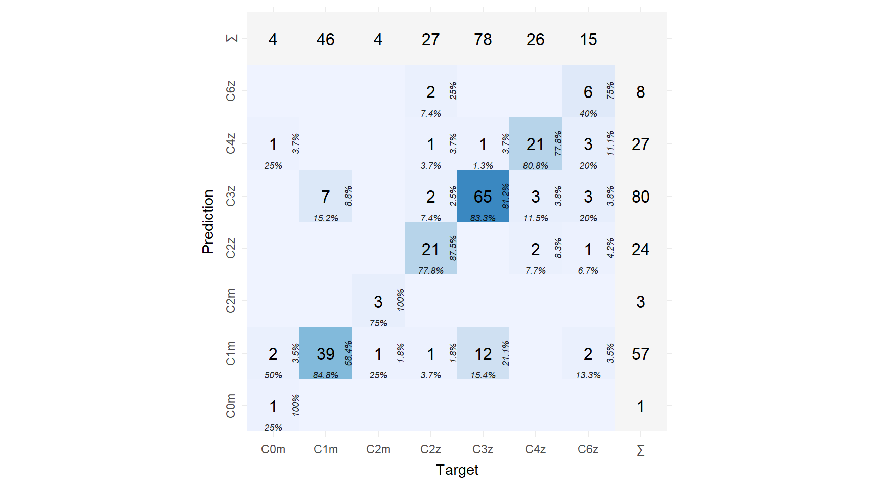
Unsurprisingly, there biggest source of confusion is distinguishing Cover 1 Man from Cover 3 Zone. Let’s take a look at some play that are labeled as Cover 1 Man but are really Cover 3 Zone (with thanks to the great package sportyR for making it easy to plot a field).
tracking <- readr::read_csv("../../../nfl-big-data-bowl-2021/input/week1.csv") %>%
  ngscleanR::clean_and_rotate() %>%
  filter(frame_id == 31)

plot_plays <- play_indices[test_id, ] %>%
  bind_cols(predictions) %>%
  filter(prediction == 2, label == 5) %>%
  select(play) %>%
  dplyr::slice(1:4) %>%
  pull(play)
plots <- map(plot_plays, ~ {
  plot <- tracking %>%
    filter(play == .x) %>%
    ngscleanR::plot_play(
      animated = FALSE,
      segment_length = 6,
      segment_size = 3,
      dot_size = 4
    )

  plot +
    theme(
      plot.title = element_blank(),
      plot.caption = element_blank(),
      plot.margin = unit(c(0, 0, 0, 0), "cm")
    )
})

combined <- (plots[[1]] + plots[[2]]) / (plots[[3]] + plots[[4]])

combined + plot_annotation(
  title = "Sample Cover 3 plays that model thinks are Cover 1",
  theme = theme(plot.title = element_text(size = 16, hjust = 0.5))
)
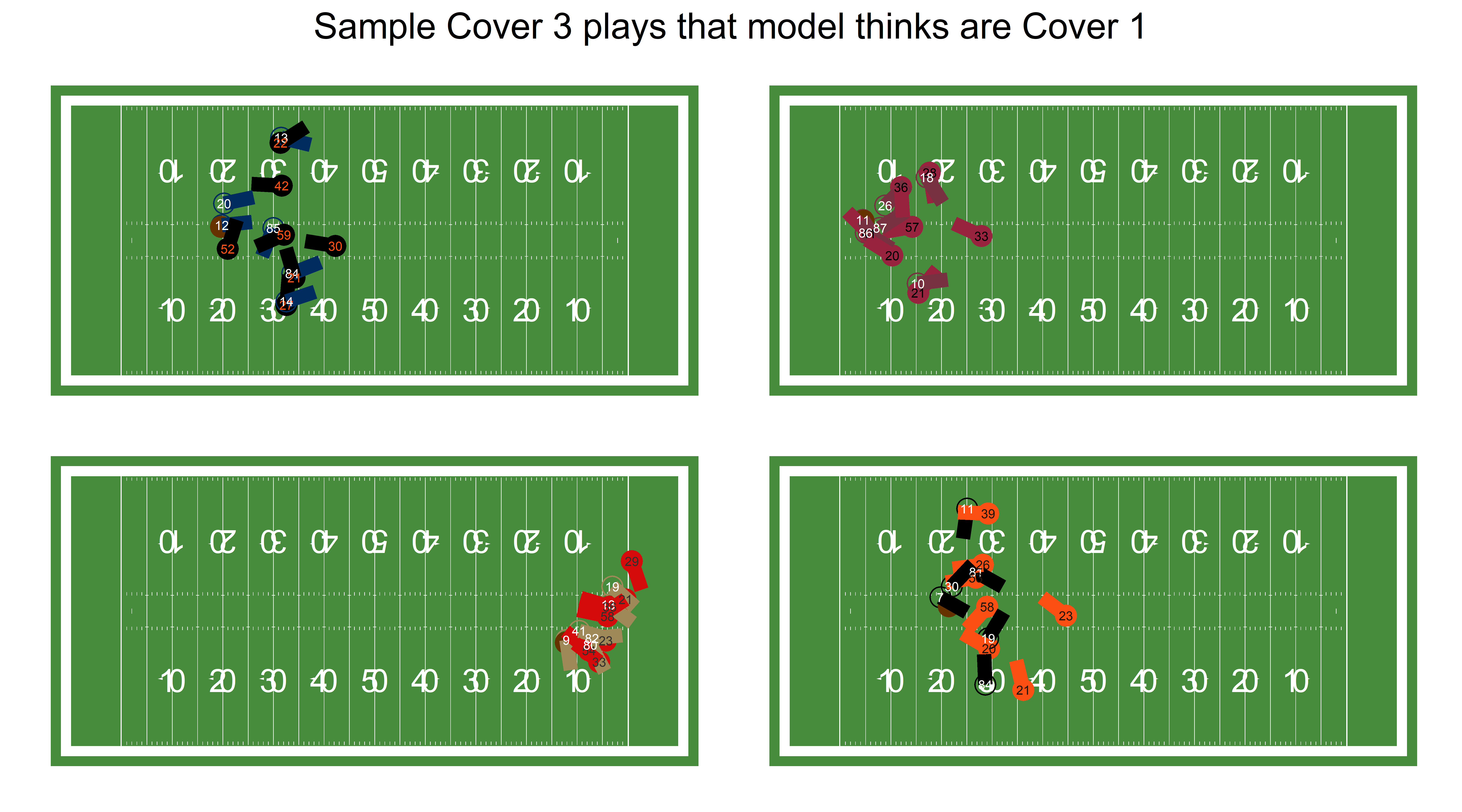
It’s kind of hard to tell from a still image exactly why the model got them wrong. The bottom right one, in particular, should be easy for a model to tell that it’s Cover 3, since so many defenders are watching the quarterback. However, the glass half full view is that it’s impressive that the model can get nearly 80% of plays right with only 1 week of data and 1 frame per play.
Wrapping Up
Hopefully this has been at least somewhat helpful to someone. We’ve covered how to get data into tensors, deal with datasets and dataloaders, augmentation, and how to train a model with k-fold cross-validation.
One thing I didn’t cover is how to deal with multiple frames per play. One option would be to feed the CNN predictions in each frame into a LSTM. Another would be to send every frame in a given play into the CNN and then perform some sort of pooling by play afterwards. I didn’t explore this in the post because (a) it’s already long enough and (b) my laptop can barely handle knitting this post at its given size and more frames would kill it.
Some things that I learned:
- If you get inexplicable error messages, make very sure that you don’t have any missing data anywhere (including in the labels)
- Be very careful with using
torch_squeeze()without any arguments (i.e., the index to squeeze) because if you happen to have a batch size of 1 at the end of an epoch, the batch size dimension will get squeezed out and break things - Kaggle supports R and comes with
torchpre-installed, BUT it’s a very old version oftorchso upgrade to the latest version in your kaggle notebook to get access to all the new things - If you have limited memory or don’t have access to a GPU on your own computer, use Kaggle to train models!
- The documentation is very helpful!
This post wouldn’t have been possible without a lot of help from a lot of people. Thank you in particular to Daniel Falbel, both for all of his work on torch and for answering a million of my questions, and to Sean Clement and Lau Sze Yui for allowing me to pester them with a million questions about neural nets. Additional thanks to helpful discussions with Timo Riske, Suvansh Sanjeev, Udit Ranasaria, Rishav Dutta, and Zach Feldman.