Gunslingers vs. Game Managers is the stupidest football argument out there. So, naturally, I love it. This post is going to quantify what gunslingers are, what game managers are, and measure these for every QB since 2005.
Gunslingers are higher risk, higher reward type of quarterbacks - typically they throw for a ton of yards, have a lot of touchdown passes, scramble and run around a lot, throw lots of deep balls, but also take negative plays, and throw interceptions. Brett Favre is the patron saint of gunslingers (unfortunately his prime gunslinging days predate the nflfastR pbp data), but players like Jameis Winston and Rex “Screw It, I’m Going Deep” Grossman are also known as gunslingers, as well.
Game Managers are lower-risk (and potentially also lower-reward) players. A game manager doesn’t make mistakes - takes very few sacks, doesn’t throw interceptions and completes a percent of their passes.
First, we load our data:
Now I just want the plays that are the QB, so all dropbacks. I am excluding designed QB runs as those exist outside the gunslinger vs game manager paradigm. I’m also going to strip out the season by taking the first 4 digits of the game id.
Now we want to summarize each QB’s performance each year: What is a Game Manager? A game manager doesn’t throw interceptions, doesn’t take sacks, doesn’t take negative plays (which we’ll measure by success rate), and complete a lot of passes.
Stats <- passes %>% filter(home_wp > 0.1, home_wp < 0.9, qb_dropback==1) %>%
           mutate(QB = ifelse(is.na(passer_player_name), rusher_player_name, passer_player_name)) %>%
           group_by(QB, year) %>%
           summarize(numDropbacks = n(),
                    passAttempts = sum(pass_attempt),
                    #Game Manager Calculations:
                    completions = sum(complete_pass),
                    completionPercent = completions / passAttempts,
                    ints = sum(interception),
                    sacks = sum(sack)/numDropbacks,
                    successRate = mean(success),

                    #Gunslinger Calculations:
                    meanAirYards = mean(air_yards, na.rm=TRUE),
                    tds = sum(touchdown),
                    shortOfSticksOnThird = sum(down==3 & air_yards < ydstogo & third_down_failed, na.rm=TRUE),
                    thirdDownDropbacks = sum(down==3, na.rm=TRUE ),
                    shortOfSticksOnThirdRate = shortOfSticksOnThird / thirdDownDropbacks,
                    passYards = sum(yards_gained[pass_attempt==1], na.rm=TRUE),
                    rushYards = sum(yards_gained[pass_attempt==0], na.rm=TRUE),
                    team = last(posteam),
                    throwAways = sum(is.na(receiver_player_name) & pass_attempt==1),
                    throwAwayRate = throwAways/numDropbacks,

                    #EPA
                    meanEPA = mean(epa),
                    sdEPA = sd(epa)
                    ) %>%
           filter(passAttempts > 200) %>%
           arrange(desc(meanEPA)) %>% mutate(ID = paste(QB, "_", year))


head(Stats)
# A tibble: 6 x 22
# Groups:   QB [3]
  QB    year  numDropbacks passAttempts completions completionPerce~
  <chr> <chr>        <int>        <dbl>       <dbl>            <dbl>
1 A.Ro~ 2011           467          435         276            0.634
2 P.Ma~ 2018           544          519         331            0.638
3 T.Br~ 2007           524          514         338            0.658
4 A.Ro~ 2020           474          455         313            0.688
5 P.Ma~ 2020           600          564         367            0.651
6 P.Ma~ 2019           529          500         322            0.644
# ... with 16 more variables: ints <dbl>, sacks <dbl>,
#   successRate <dbl>, meanAirYards <dbl>, tds <dbl>,
#   shortOfSticksOnThird <int>, thirdDownDropbacks <int>,
#   shortOfSticksOnThirdRate <dbl>, passYards <dbl>, rushYards <dbl>,
#   team <chr>, throwAways <int>, throwAwayRate <dbl>, meanEPA <dbl>,
#   sdEPA <dbl>, ID <chr>
Okay so now lets combine all these into one “gunslinger” score. We’ll standardize each variable so it has a mean of 0 and a standard deviation of 1, using the scale() command. I then weight each feature by how important I think this is:
TD passes - weight 75% Deep Passes (average air yards) - weight 100% Scramble Yards - weight 25% Not throwing short of Sticks on Third - weight 75% Lots of pass yards - weight 75%
Gunslinger <- Stats %>% select(QB, year, tds, passYards, meanAirYards, rushYards, shortOfSticksOnThirdRate, team)
cols <- c('tds', 'passYards', 'rushYards', 'shortOfSticksOnThirdRate', 'meanAirYards')
tdWeight <- 0.75
passWeight <- 0.5
rushWeight <- 0.25
shortWeight <- 0.75
airWeight <- 1
Gunslinger[cols] <- scale(Gunslinger[cols])
Gunslinger <- Gunslinger %>% mutate(GunslingScore = tdWeight* tds + passWeight* passYards + rushWeight* rushYards - shortWeight * shortOfSticksOnThirdRate + airWeight* meanAirYards) %>%  arrange(-GunslingScore)
Gunslinger$GunslingScore <- scale(Gunslinger$GunslingScore)
And now for game managers:
Don’t throw interceptions - 100% High success rate (no negative plays) - 70% Don’t take sacks - 50% High completion rate - 75%
Manager <- Stats %>% select(QB, year, ints, successRate, sacks, completionPercent, team, meanEPA, sdEPA)
cols <- c('ints', 'successRate', 'sacks', 'completionPercent')
Manager[cols] <- scale(Manager[cols])
intWeight <- 1
successWeight <- 0.70
sacksWeight <- 0.50
completeWeight <- 75
Manager <- Manager %>% mutate(ManageScore = -1*ints*intWeight + successRate*successWeight - sacks*sacksWeight + completionPercent*completeWeight) %>%  arrange(-ManageScore)
Manager$ManageScore <- scale(Manager$ManageScore)
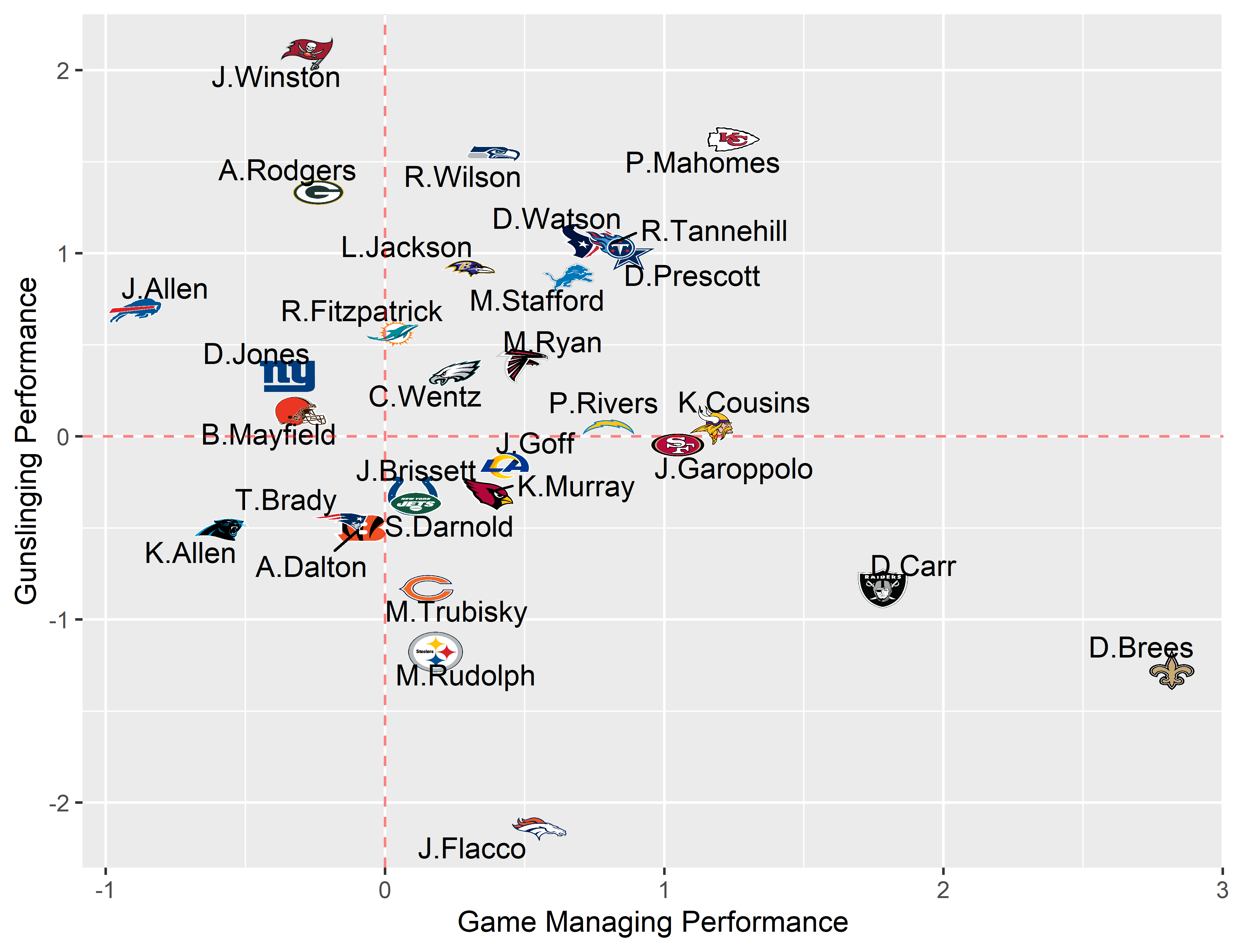
Now we joing them together and plot them. To keep the graph from getting cluttered, I’m just plotting 2019.
Looking at this graph, quarterbacks in the upper left are true “gunslingers” - high performance as gunslingers, and low performance as game managers. Players in the bottom right are pure game managers. Quarterbacks in the upper right are just really good, while those in the lower left are just not very good at anything.
Jameis Winston is a great gunslinger, but a terrible game manager, and to a lesser extent, so was Aaron Rodgers. Drew Brees, however, is a great game manager, and not much of a gunslinger anymore. In the upper right, Pat Mahomes is really good at everything.
library(nflfastR)
library(ggrepel)
library(ggimage)


Combined <- Gunslinger %>% left_join(Manager) %>%  left_join(teams_colors_logos, by = c('team' = 'team_abbr')) %>% arrange(-GunslingScore)

Combined %>% filter(year == 2019) %>%  ggplot(aes(x=ManageScore, y=GunslingScore, label=QB)) +
  geom_image(aes(image = team_logo_espn)) +
  geom_text_repel(aes(label=QB)) +
  geom_hline(yintercept = 0, color = "red", linetype = "dashed", alpha=0.5) +
  geom_vline(xintercept =  0, color = "red", linetype = "dashed", alpha=0.5) +
  labs(x = "Game Managing Performance", y="Gunslinging Performance")
If you disagree with my weights, I have a shiny app where you can change them and generate your own scores: https://davidranderson.shinyapps.io/GunslingersVsGameManagers/