About
This page describes the nflfastR models before showing that they are well calibrated using the procedure introduced by Yurko, Ventura, and Horowitz. Because the 2020 season will mark 22 seasons of nflfastR data, the main purpose behind creating new models for EP and WP was to build in era adjustments to fascilitate better cross-era comparisons. However, we also discovered that switching to tree-based methods could improve model calibration, especially for end-of-half situations with complicated nonlinear interactions between variables. Because we are introducing new models, we compare our calibration results to nflscrapR to show that these new models are somewhat better calibrated. If they weren’t, there would be no point in updating the models!
nflfastR switching from the nflscrapR EP and WP models to its own model should not be thought of as a criticism of nflscrapR: the improvements are relatively minor and nflscrapR provided the code base to perform much of this analysis, breaking new ground in the process.
Model features
The models are trained using xgboost, which uses training data to create decision trees.
EP model features
- Seconds remaining in half
- Yard line
- Whether possession team is at home
- Roof type: retractable, dome, or outdoors
- Down
- Yards to go
- Era: 1999-2001 (pre-expansion), 2002-2005 (pre-CPOE), 2006-2013 (pre-LOB rules change), 2014-2017, 2018 and beyond
- Timeouts remaining for each team
WP model features
- Seconds remaining in half
- Seconds remaining in game
- Yard line
- Score differential
- Ratio of point differential: \[\mathrm{diff\_time\_ratio}=\mathrm{point\_differential}\cdot e^{4\cdot\frac{3600-\mathrm{game\_seconds\_remaining}}{3600}}\]
- Down
- Yards to go
- Timeouts remaining for each team
- Whether team will receive 2nd half kickoff
- Whether possession team is at home
- Model with Vegas line only: \[\mathrm{spread\_time}=\mathrm{posteam\_spread}\cdot e^{-4\cdot\frac{3600-\mathrm{game\_seconds\_remaining}}{3600}}\]
CP and expected yards after the catch model features
- Yard line
- Whether possession team is at home
- Roof type: retractable, dome, or outdoors
- Down
- Yards to go
- Distance to sticks (air yards - yards to go)
- Era: 2006-2013, 2014-2017, 2018 and beyond (note that air yards data only go back to 2006, so there is no CP for earlier years)
- Air yards
- Whether air yards is 0 (probably unnecessary with tree-based method and a relic from earlier models where it was included because completion percentage is much lower for 0 air yard passes)
- Pass location (binary: middle or not middle)
- Whether quarterback was hit on the play
- For xyac model only: how far away the goal line is when the ball is caught
Expected dropback model features
- Yard line
- Whether possession team is at home
- Roof type: retractable, dome, or outdoors
- Down
- Quarter
- Half seconds remaining
- Yards to go
- Score differential
- Timeouts remaining for each team
- Win probability (both with spread and non-spread adjusted)
- Era: 2006-2013, 2014-2017, 2018 and beyond (note that scramble data only go back to 2006, so there is no xpass for earlier years)
EP Model Calibration Results
The goal of this section is to show that the nflfastR EP model is well calibrated. To measure calibration, we follow Yurko et al. and perform leave-one-season-out (LOSO) calibration. In particular, for each of the 20 available seasons (2000-2019), we exclude one season, train the EP model on the other 19 seasons, and then compare the model’s predictions in the holdout season to what actually happened in that season. If the model is well calibrated, we would expect that, for example, 50 percent of plays with a touchdown probability of 50 percent prior to the play would have the next score be a touchdown for the possession team.
Let’s start with some setup. The file used here isn’t pushed because it’s large, but its creation can be seen here and the file can be accessed here.
set.seed(2013) # GoHawks
library(tidyverse)
library(xgboost)

# some helper files are in these
source("https://raw.githubusercontent.com/mrcaseb/nflfastR/master/R/helper_add_nflscrapr_mutations.R")
source("https://raw.githubusercontent.com/mrcaseb/nflfastR/master/R/helper_add_ep_wp.R")
source("https://raw.githubusercontent.com/mrcaseb/nflfastR/master/R/helper_add_cp_cpoe.R")

# from remote
pbp_data <- readRDS(url("https://github.com/guga31bb/nflfastR-data/blob/master/models/cal_data.rds?raw=true"))

# from local
# pbp_data <- readRDS('../../nflfastR-data/models/cal_data.rds')

model_data <- pbp_data %>%
  # in 'R/helper_add_nflscrapr_mutations.R'
  make_model_mutations() %>%
  mutate(
    label = case_when(
      Next_Score_Half == "Touchdown" ~ 0,
      Next_Score_Half == "Opp_Touchdown" ~ 1,
      Next_Score_Half == "Field_Goal" ~ 2,
      Next_Score_Half == "Opp_Field_Goal" ~ 3,
      Next_Score_Half == "Safety" ~ 4,
      Next_Score_Half == "Opp_Safety" ~ 5,
      Next_Score_Half == "No_Score" ~ 6
    ),
    label = as.factor(label),
    # use nflscrapR weights
    Drive_Score_Dist = Drive_Score_Half - drive,
    Drive_Score_Dist_W = (max(Drive_Score_Dist) - Drive_Score_Dist) /
      (max(Drive_Score_Dist) - min(Drive_Score_Dist)),
    ScoreDiff_W = (max(abs(score_differential), na.rm = T) - abs(score_differential)) /
      (max(abs(score_differential), na.rm = T) - min(abs(score_differential), na.rm = T)),
    Total_W = Drive_Score_Dist_W + ScoreDiff_W,
    Total_W_Scaled = (Total_W - min(Total_W, na.rm = T)) /
      (max(Total_W, na.rm = T) - min(Total_W, na.rm = T))
  ) %>%
  filter(
    !is.na(defteam_timeouts_remaining), !is.na(posteam_timeouts_remaining),
    !is.na(yardline_100)
  ) %>%
  select(
    label,
    season,
    half_seconds_remaining,
    yardline_100,
    home,
    retractable,
    dome,
    outdoors,
    ydstogo,
    era0, era1, era2, era3, era4,
    down1, down2, down3, down4,
    posteam_timeouts_remaining,
    defteam_timeouts_remaining,
    Total_W_Scaled
  )

# idk why this is all necessary for xgb but it is
model_data <- model_data %>%
  mutate(
    label = as.numeric(label),
    label = label - 1
  )

rm(pbp_data)

seasons <- unique(model_data$season)
Input the stuff we’ll need to fit the model. The parameters were obtained from cross-validation, where each season was forced to be entirely contained in a given CV fold to prevent leakage in labels from one fold to another (for example, if a given drive were split up between folds).
Now do the LOSO model fitting.
cv_results <- map_dfr(seasons, function(x) {
  test_data <- model_data %>%
    filter(season == x) %>%
    select(-season)
  train_data <- model_data %>%
    filter(season != x) %>%
    select(-season)

  full_train <- xgboost::xgb.DMatrix(model.matrix(~ . + 0, data = train_data %>% select(-label, -Total_W_Scaled)),
    label = train_data$label, weight = train_data$Total_W_Scaled
  )
  ep_model <- xgboost::xgboost(params = params, data = full_train, nrounds = nrounds, verbose = 2)

  preds <- as.data.frame(
    matrix(predict(ep_model, as.matrix(test_data %>% select(-label, -Total_W_Scaled))), ncol = 7, byrow = TRUE)
  )
  colnames(preds) <- c(
    "Touchdown", "Opp_Touchdown", "Field_Goal", "Opp_Field_Goal",
    "Safety", "Opp_Safety", "No_Score"
  )

  cv_data <- bind_cols(test_data, preds) %>% mutate(season = x)
  return(cv_data)
})

# get the BINS for the calibration plot
plot <- cv_results %>%
  select(Touchdown, Opp_Touchdown, Field_Goal, Opp_Field_Goal, Safety, Opp_Safety, No_Score, label) %>%
  pivot_longer(-label, names_to = "type", values_to = "pred_prob") %>%
  mutate(bin_pred_prob = round(pred_prob / 0.05) * .05) %>%
  mutate(outcome = case_when(
    label == 0 ~ "Touchdown",
    label == 1 ~ "Opp_Touchdown",
    label == 2 ~ "Field_Goal",
    label == 3 ~ "Opp_Field_Goal",
    label == 4 ~ "Safety",
    label == 5 ~ "Opp_Safety",
    label == 6 ~ "No_Score"
  )) %>%
  group_by(type, bin_pred_prob) %>%
  mutate(correct = if_else(outcome == type, 1, 0)) %>%
  summarize(
    n_plays = n(),
    n_outcome = sum(correct),
    bin_actual_prob = n_outcome / n_plays
  )
Here is the EP calibration plot. Points close to the diagonal dotted line are consistent with a well-calibrated model:
ann_text <- data.frame(
  x = c(.25, 0.75), y = c(0.75, 0.25),
  lab = c("More times\nthan expected", "Fewer times\nthan expected"),
  next_score_type = factor("No Score (0)")
)
plot %>%
  # about .75M plays in total
  # filter(n_plays >= 50) %>%
  ungroup() %>%
  mutate(
    type = fct_relevel(
      type,
      "Opp_Safety", "Opp_Field_Goal",
      "Opp_Touchdown", "No_Score", "Safety",
      "Field_Goal", "Touchdown"
    ),
    type = fct_recode(type,
      "-Field Goal (-3)" = "Opp_Field_Goal",
      "-Safety (-2)" = "Opp_Safety",
      "-Touchdown (-7)" = "Opp_Touchdown",
      "Field Goal (3)" = "Field_Goal",
      "No Score (0)" = "No_Score",
      "Touchdown (7)" = "Touchdown",
      "Safety (2)" = "Safety"
    )
  ) %>%
  ggplot() +
  geom_point(aes(x = bin_pred_prob, y = bin_actual_prob, size = n_plays)) +
  geom_smooth(aes(x = bin_pred_prob, y = bin_actual_prob), method = "loess") +
  geom_abline(slope = 1, intercept = 0, color = "black", lty = 2) +
  coord_equal() +
  scale_x_continuous(limits = c(0, 1)) +
  scale_y_continuous(limits = c(0, 1)) +
  labs(
    size = "Number of plays",
    x = "Estimated next score probability",
    y = "Observed next score probability"
  ) +
  geom_text(data = ann_text, aes(x = x, y = y, label = lab), size = 2) +
  theme_bw() +
  theme(
    plot.title = element_text(hjust = 0.5),
    strip.background = element_blank(),
    strip.text = element_text(size = 12),
    axis.title = element_text(size = 12),
    axis.text.y = element_text(size = 12),
    axis.text.x = element_text(size = 10, angle = 90),
    legend.title = element_text(size = 12),
    legend.text = element_text(size = 12),
    legend.position = c(1, .05), legend.justification = c(1, 0)
  ) +
  facet_wrap(~type, ncol = 4)
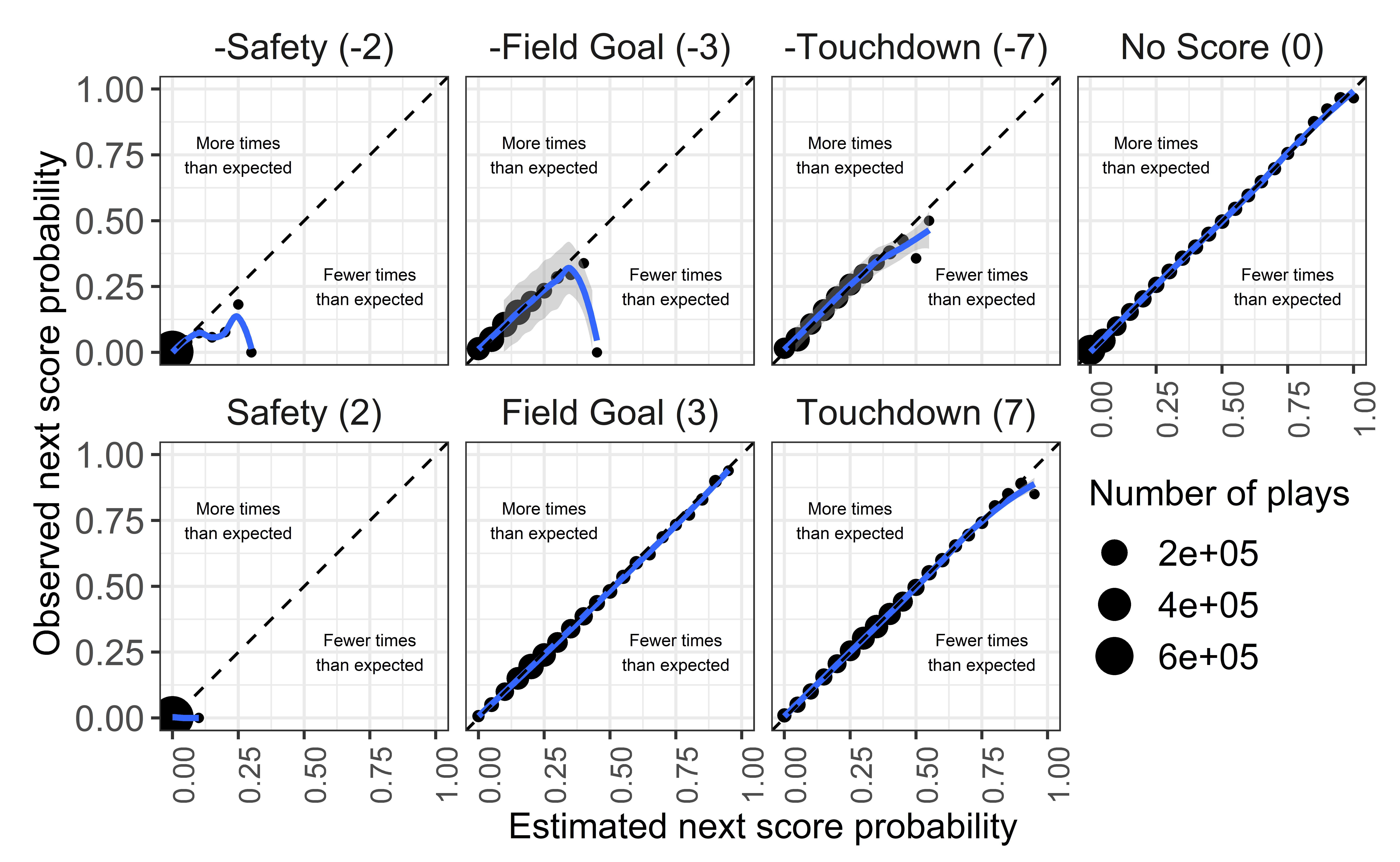
There is some weirdness with the opponent safety predictions, but these dots represent an extremely small number of plays (10-50 plays out of about 750,000).
Now let’s get the calibration error using the measure developed in Yurko et al., and compare it to nflscrapR. First we need to get the nflscrapR predictions, which we have saved from the previous version of nflfastR which applied the nflscrapR models.
# calibration error
cv_cal_error <- plot %>%
  ungroup() %>%
  mutate(cal_diff = abs(bin_pred_prob - bin_actual_prob)) %>%
  group_by(type) %>%
  summarize(
    weight_cal_error = weighted.mean(cal_diff, n_plays, na.rm = TRUE),
    n_scoring_event = sum(n_outcome, na.rm = TRUE)
  )

pbp_data <- readRDS(url("https://github.com/guga31bb/nflfastR-data/blob/master/models/cal_data_nflscrapr.rds?raw=true"))
# nflscrapr calibration error
nflscrapr <- pbp_data %>%
  select(td_prob, opp_td_prob, fg_prob, opp_fg_prob, safety_prob, opp_safety_prob, no_score_prob, Next_Score_Half) %>%
  pivot_longer(-Next_Score_Half, names_to = "type", values_to = "pred_prob") %>%
  mutate(bin_pred_prob = round(pred_prob / 0.05) * .05) %>%
  mutate(
    outcome = Next_Score_Half,
    type = case_when(
      type == "td_prob" ~ "Touchdown",
      type == "fg_prob" ~ "Field_Goal",
      type == "opp_td_prob" ~ "Opp_Touchdown",
      type == "opp_fg_prob" ~ "Opp_Field_Goal",
      type == "safety_prob" ~ "Safety",
      type == "opp_safety_prob" ~ "Opp_Safety",
      type == "no_score_prob" ~ "No_Score"
    )
  ) %>%
  group_by(type, bin_pred_prob) %>%
  mutate(correct = if_else(outcome == type, 1, 0)) %>%
  summarize(
    n_plays = n(),
    n_outcome = sum(correct),
    bin_actual_prob = n_outcome / n_plays
  ) %>%
  ungroup() %>%
  mutate(cal_diff = abs(bin_pred_prob - bin_actual_prob)) %>%
  group_by(type) %>%
  summarize(
    weight_cal_error = weighted.mean(cal_diff, n_plays, na.rm = TRUE),
    n_scoring_event = sum(n_outcome, na.rm = TRUE)
  )
rm(pbp_data)

glue::glue(
  "
--CALIBRATION ERROR--

nflfastR:
{round(with(cv_cal_error, weighted.mean(weight_cal_error, n_scoring_event)), 4)}

nflscrapR:
{round(with(nflscrapr, weighted.mean(weight_cal_error, n_scoring_event)), 4)}
"
)
--CALIBRATION ERROR--

nflfastR:
0.006

nflscrapR:
0.017
We see that the new EP model is better calibrated. Note that nflscrapR reports a calibration error of 0.01309723. The number is higher here because of the additional seasons included outside of the time period nflscrapR was trained on, and the lack of era adjustment in nflscrapR.
WP Model Calibration Results
As with EP, do some initial setup to get the data ready for fitting.
model_data <-
  readRDS(url("https://github.com/guga31bb/metrics/blob/master/wp_tuning/cal_data.rds?raw=true")) %>%
  filter(Winner != "TIE") %>%
  make_model_mutations() %>%
  prepare_wp_data() %>%
  mutate(label = ifelse(posteam == Winner, 1, 0)) %>%
  filter(
    !is.na(ep), !is.na(score_differential), !is.na(play_type), !is.na(label),
    !is.na(defteam_timeouts_remaining), !is.na(posteam_timeouts_remaining),
    !is.na(yardline_100), qtr <= 4
  ) %>%
  select(
    label,
    receive_2h_ko,
    spread_time,
    home,
    half_seconds_remaining,
    game_seconds_remaining,
    Diff_Time_Ratio,
    score_differential,
    down,
    ydstogo,
    yardline_100,
    posteam_timeouts_remaining,
    defteam_timeouts_remaining,
    season,
    # only needed for the plots here, not used in model
    qtr
  )

nrounds <- 65
params <-
  list(
    booster = "gbtree",
    objective = "binary:logistic",
    eval_metric = c("logloss"),
    eta = 0.2,
    gamma = 0,
    subsample = 0.8,
    colsample_bytree = 0.8,
    max_depth = 4,
    min_child_weight = 1
  )

seasons <- unique(model_data$season)
Do the LOSO fitting:
cv_results <- map_dfr(seasons, function(x) {
  test_data <- model_data %>%
    filter(season == x) %>%
    select(-season)
  train_data <- model_data %>%
    filter(season != x) %>%
    select(-season)

  full_train <- xgboost::xgb.DMatrix(model.matrix(~ . + 0, data = train_data %>% select(-label, -qtr, -spread_time)),
    label = train_data$label
  )
  wp_model <- xgboost::xgboost(params = params, data = full_train, nrounds = nrounds, verbose = 2)

  preds <- as.data.frame(
    matrix(predict(wp_model, as.matrix(test_data %>% select(-label, -qtr, -spread_time))))
  ) %>%
    dplyr::rename(wp = V1)

  cv_data <- bind_cols(test_data, preds) %>% mutate(season = x)
  return(cv_data)
})

# TIME FOR BINNING
wp_cv_loso_calibration_results <- cv_results %>%
  # Create BINS for wp:
  mutate(bin_pred_prob = round(wp / 0.05) * .05) %>%
  # Group by both the qtr and bin_pred_prob:
  group_by(qtr, bin_pred_prob) %>%
  # Calculate the calibration results:
  summarize(
    n_plays = n(),
    n_wins = length(which(label == 1)),
    bin_actual_prob = n_wins / n_plays
  )
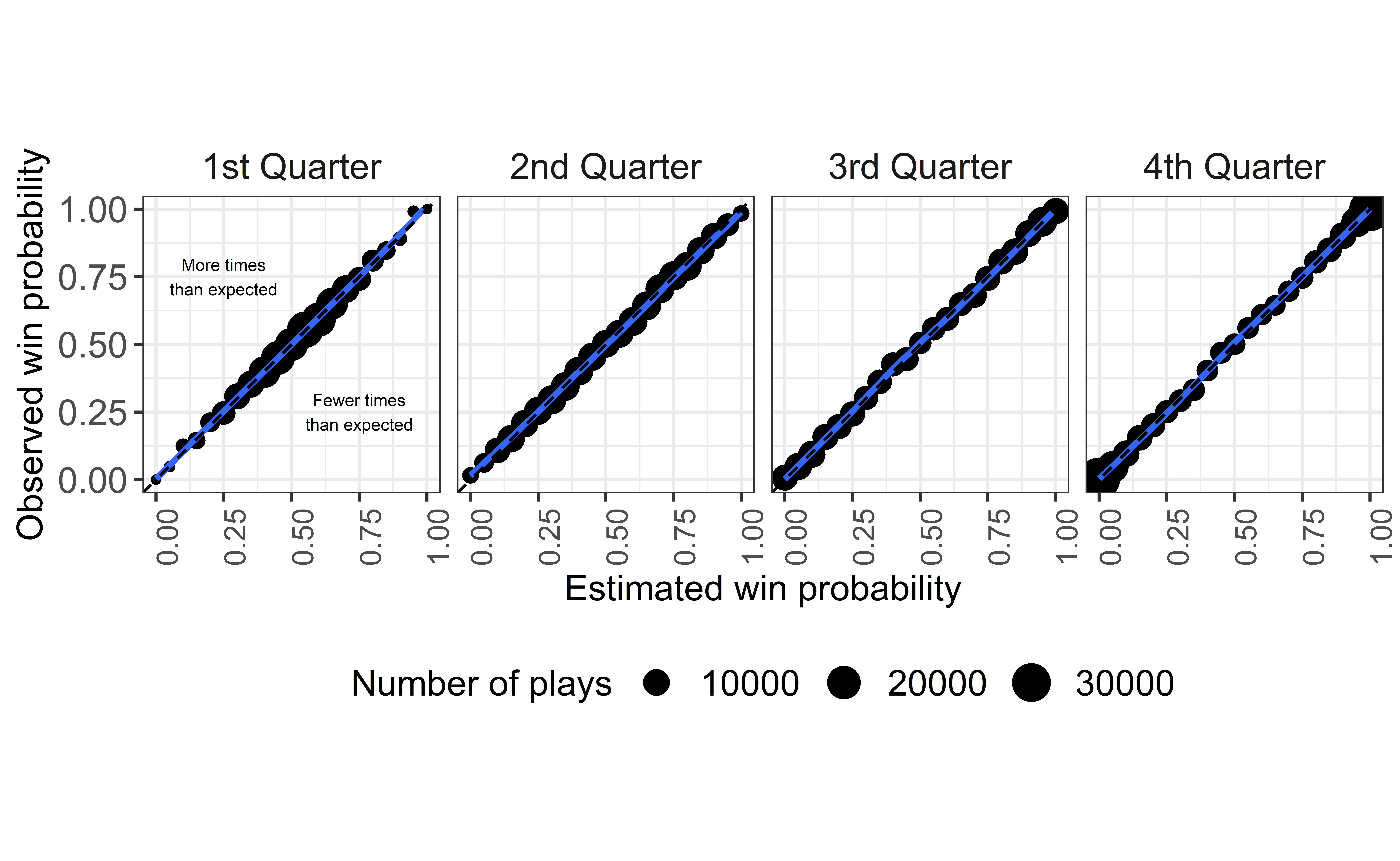
The WP plot. Looks good!
# Create a label data frame for the chart:
ann_text <- data.frame(
  x = c(.25, 0.75), y = c(0.75, 0.25),
  lab = c("More times\nthan expected", "Fewer times\nthan expected"),
  qtr = factor("1st Quarter")
)

# Create the calibration chart:
wp_cv_loso_calibration_results %>%
  ungroup() %>%
  mutate(qtr = fct_recode(factor(qtr),
    "1st Quarter" = "1", "2nd Quarter" = "2",
    "3rd Quarter" = "3", "4th Quarter" = "4"
  )) %>%
  ggplot() +
  geom_point(aes(x = bin_pred_prob, y = bin_actual_prob, size = n_plays)) +
  geom_smooth(aes(x = bin_pred_prob, y = bin_actual_prob), method = "loess") +
  geom_abline(slope = 1, intercept = 0, color = "black", lty = 2) +
  coord_equal() +
  scale_x_continuous(limits = c(0, 1)) +
  scale_y_continuous(limits = c(0, 1)) +
  labs(
    size = "Number of plays",
    x = "Estimated win probability",
    y = "Observed win probability"
  ) +
  geom_text(data = ann_text, aes(x = x, y = y, label = lab), size = 2) +
  theme_bw() +
  theme(
    plot.title = element_text(hjust = 0.5),
    strip.background = element_blank(),
    strip.text = element_text(size = 12),
    axis.title = element_text(size = 12),
    axis.text.y = element_text(size = 12),
    axis.text.x = element_text(size = 10, angle = 90),
    legend.title = element_text(size = 12),
    legend.text = element_text(size = 12),
    legend.position = "bottom"
  ) +
  facet_wrap(~qtr, ncol = 4)
And get the WP calibration error:
# Calculate the calibration error values:
wp_cv_cal_error <- wp_cv_loso_calibration_results %>%
  ungroup() %>%
  mutate(cal_diff = abs(bin_pred_prob - bin_actual_prob)) %>%
  group_by(qtr) %>%
  summarize(
    weight_cal_error = weighted.mean(cal_diff, n_plays, na.rm = TRUE),
    n_wins = sum(n_wins, na.rm = TRUE)
  )

# get nflscrapR to compare
pbp_data <- readRDS(url("https://github.com/guga31bb/nflfastR-data/blob/master/models/cal_data_nflscrapr.rds?raw=true")) %>%
  mutate(label = ifelse(posteam == Winner, 1, 0)) %>%
  filter(qtr <= 4, !is.na(label), !is.na(posteam), !is.na(wp))

nflscrapR <- pbp_data %>%
  # Create binned probability column:
  mutate(bin_pred_prob = round(wp / 0.05) * .05) %>%
  # Group by both the qtr and bin_pred_prob:
  group_by(qtr, bin_pred_prob) %>%
  # Calculate the calibration results:
  summarize(
    n_plays = n(),
    n_wins = length(which(label == 1)),
    bin_actual_prob = n_wins / n_plays
  ) %>%
  ungroup() %>%
  mutate(cal_diff = abs(bin_pred_prob - bin_actual_prob)) %>%
  group_by(qtr) %>%
  summarize(
    weight_cal_error = weighted.mean(cal_diff, n_plays, na.rm = TRUE),
    n_wins = sum(n_wins, na.rm = TRUE)
  )

glue::glue(
  "--CALIBRATION ERROR--

nflfastR:
{round(with(wp_cv_cal_error, weighted.mean(weight_cal_error, n_wins)), 4)}

nflscrapR:
{round(with(nflscrapR, weighted.mean(weight_cal_error, n_wins)), 4)}"
)
--CALIBRATION ERROR--

nflfastR:
0.0055

nflscrapR:
0.0397
Again, the new WP model represents an improvement.
WP Model Calibration Results: with point spread
nflfastR has a secondary win probability model that also incorporates the pregame spread to more accurately reflect a team’s chances of winning. Below are calibration results for this model.
Do the LOSO fitting:
cv_results <- map_dfr(seasons, function(x) {
  test_data <- model_data %>%
    filter(season == x) %>%
    select(-season)
  train_data <- model_data %>%
    filter(season != x) %>%
    select(-season)

  full_train <- xgboost::xgb.DMatrix(model.matrix(~ . + 0, data = train_data %>% select(-label, -qtr)),
    label = train_data$label
  )
  wp_model <- xgboost::xgboost(params = params, data = full_train, nrounds = nrounds, verbose = 2)

  preds <- as.data.frame(
    matrix(predict(wp_model, as.matrix(test_data %>% select(-label, -qtr))))
  ) %>%
    dplyr::rename(wp = V1)

  cv_data <- bind_cols(test_data, preds) %>% mutate(season = x)
  return(cv_data)
})

# TIME FOR BINNING
wp_cv_loso_calibration_results <- cv_results %>%
  # Create BINS for wp:
  mutate(bin_pred_prob = round(wp / 0.05) * .05) %>%
  # Group by both the qtr and bin_pred_prob:
  group_by(qtr, bin_pred_prob) %>%
  # Calculate the calibration results:
  summarize(
    n_plays = n(),
    n_wins = length(which(label == 1)),
    bin_actual_prob = n_wins / n_plays
  )
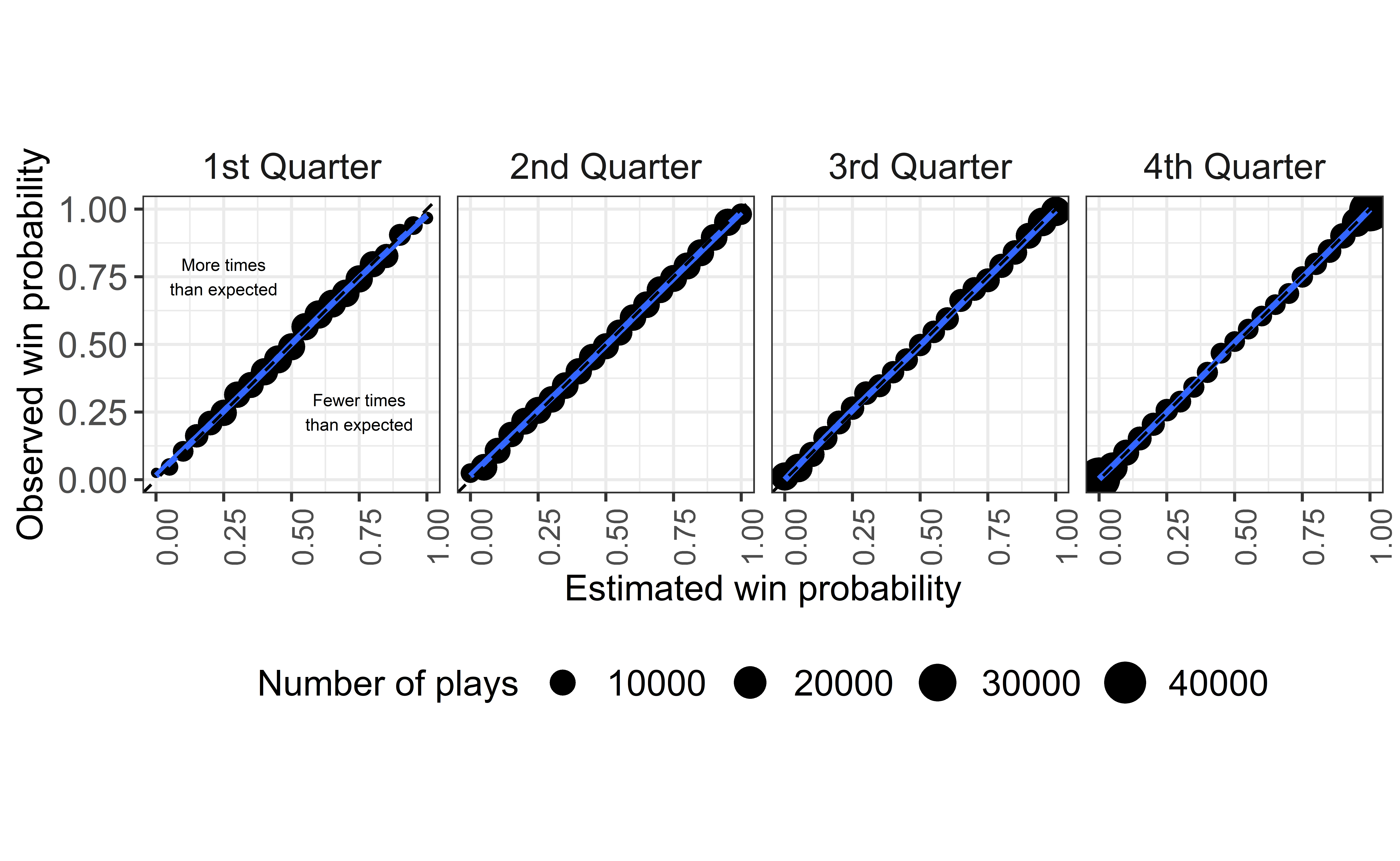
The WP plot.
# Create a label data frame for the chart:
ann_text <- data.frame(
  x = c(.25, 0.75), y = c(0.75, 0.25),
  lab = c("More times\nthan expected", "Fewer times\nthan expected"),
  qtr = factor("1st Quarter")
)

# Create the calibration chart:
wp_cv_loso_calibration_results %>%
  ungroup() %>%
  mutate(qtr = fct_recode(factor(qtr),
    "1st Quarter" = "1", "2nd Quarter" = "2",
    "3rd Quarter" = "3", "4th Quarter" = "4"
  )) %>%
  ggplot() +
  geom_point(aes(x = bin_pred_prob, y = bin_actual_prob, size = n_plays)) +
  geom_smooth(aes(x = bin_pred_prob, y = bin_actual_prob), method = "loess") +
  geom_abline(slope = 1, intercept = 0, color = "black", lty = 2) +
  coord_equal() +
  scale_x_continuous(limits = c(0, 1)) +
  scale_y_continuous(limits = c(0, 1)) +
  labs(
    size = "Number of plays",
    x = "Estimated win probability",
    y = "Observed win probability"
  ) +
  geom_text(data = ann_text, aes(x = x, y = y, label = lab), size = 2) +
  theme_bw() +
  theme(
    plot.title = element_text(hjust = 0.5),
    strip.background = element_blank(),
    strip.text = element_text(size = 12),
    axis.title = element_text(size = 12),
    axis.text.y = element_text(size = 12),
    axis.text.x = element_text(size = 10, angle = 90),
    legend.title = element_text(size = 12),
    legend.text = element_text(size = 12),
    legend.position = "bottom"
  ) +
  facet_wrap(~qtr, ncol = 4)
And get the WP calibration error:
# Calculate the calibration error values:
wp_cv_cal_error <- wp_cv_loso_calibration_results %>%
  ungroup() %>%
  mutate(cal_diff = abs(bin_pred_prob - bin_actual_prob)) %>%
  group_by(qtr) %>%
  summarize(
    weight_cal_error = weighted.mean(cal_diff, n_plays, na.rm = TRUE),
    n_wins = sum(n_wins, na.rm = TRUE)
  )
glue::glue(
  "--CALIBRATION ERROR--

nflfastR with Vegas line:
{round(with(wp_cv_cal_error, weighted.mean(weight_cal_error, n_wins)), 4)}

nflscrapR:
{round(with(nflscrapR, weighted.mean(weight_cal_error, n_wins)), 4)}"
)
--CALIBRATION ERROR--

nflfastR with Vegas line:
0.0066

nflscrapR:
0.0397
Again, the new WP model is better calibrated than nflscrapR. In our testing, incorporating the spread substantially improved the performance of the model as measured by cross-validation classification accuracy (reduced error rate from 27% to 23%) and log loss (reduced from .52 to .44). We include a time-decaying function of spread on its own as including spread on its own increases the LOSO calibration error, especially in the fourth quarter. We also tried removing the home indicator in the spread model, but this worsened the calibration results. Adding the over/under also worsened calibration results.
CP Model Calibration Results
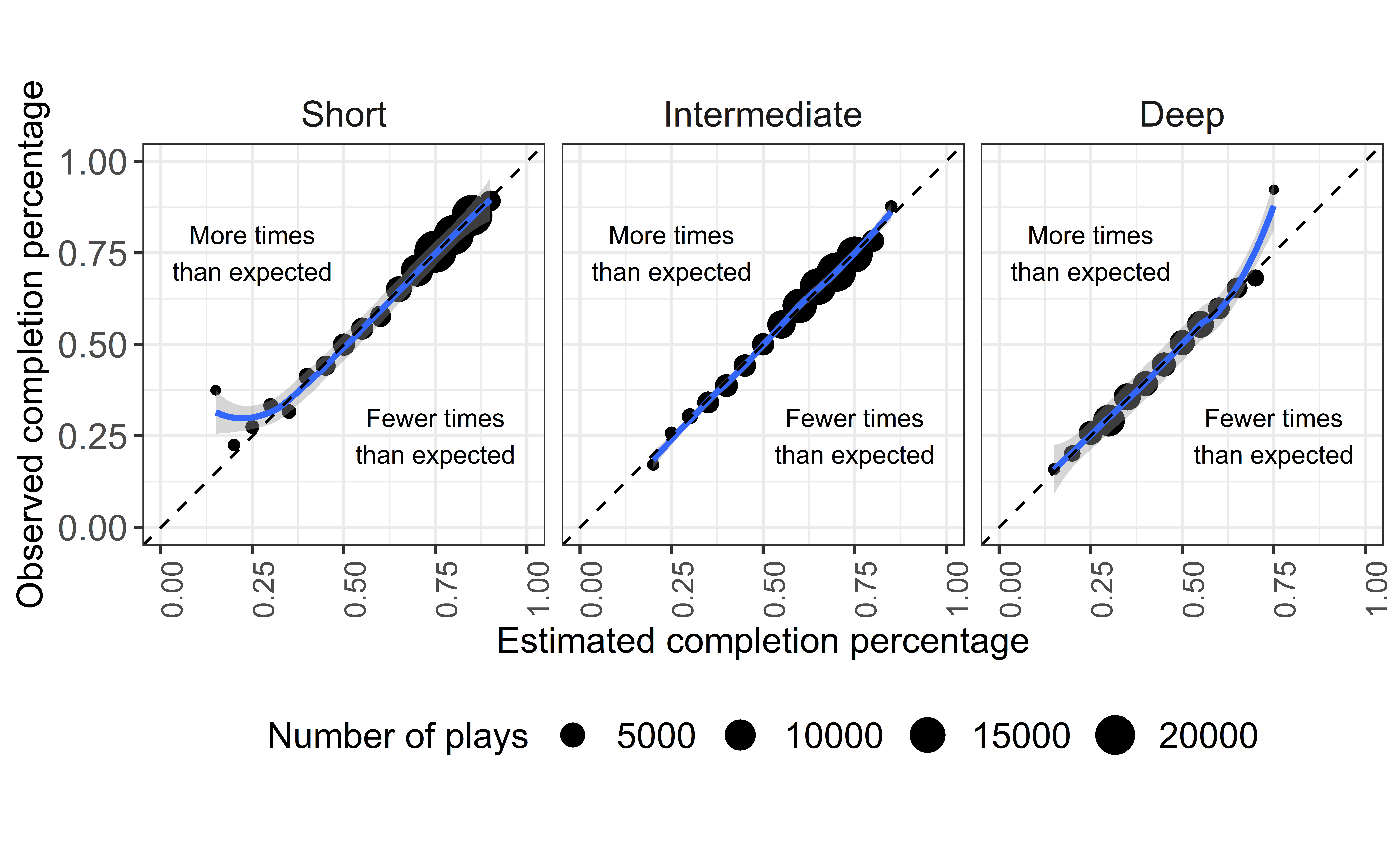
By now, the process should be familiar.
pbp <- readRDS(url("https://github.com/guga31bb/nflfastR-data/blob/master/models/cal_data.rds?raw=true"))

model_data <- pbp %>%
  filter(season >= 2006) %>%
  make_model_mutations() %>%
  dplyr::mutate(
    receiver_player_name =
      stringr::str_extract(desc, "(?<=((to)|(for))\\s[:digit:]{0,2}\\-{0,1})[A-Z][A-z]*\\.\\s?[A-Z][A-z]+(\\s(I{2,3})|(IV))?"),
    pass_middle = dplyr::if_else(pass_location == "middle", 1, 0),
    air_is_zero = dplyr::if_else(air_yards == 0, 1, 0),
    distance_to_sticks = air_yards - ydstogo
  ) %>%
  dplyr::filter(complete_pass == 1 | incomplete_pass == 1 | interception == 1) %>%
  dplyr::filter(!is.na(air_yards) & air_yards >= -15 & air_yards < 70 & !is.na(receiver_player_name) & !is.na(pass_location)) %>%
  dplyr::select(
    season, complete_pass, air_yards, yardline_100, ydstogo,
    down1, down2, down3, down4, air_is_zero, pass_middle,
    era2, era3, era4, qb_hit, home,
    outdoors, retractable, dome, distance_to_sticks
  )
rm(pbp)

seasons <- unique(model_data$season)


nrounds <- 560
params <-
  list(
    booster = "gbtree",
    objective = "binary:logistic",
    eval_metric = c("logloss"),
    eta = 0.025,
    gamma = 5,
    subsample = 0.8,
    colsample_bytree = 0.8,
    max_depth = 4,
    min_child_weight = 6,
    base_score = mean(model_data$complete_pass)
  )

cv_results <- map_dfr(2006:2019, function(x) {
  test_data <- model_data %>%
    filter(season == x) %>%
    select(-season)
  train_data <- model_data %>%
    filter(season != x) %>%
    select(-season)

  full_train <- xgboost::xgb.DMatrix(model.matrix(~ . + 0, data = train_data %>% select(-complete_pass)),
    label = train_data$complete_pass
  )
  cp_model <- xgboost::xgboost(params = params, data = full_train, nrounds = nrounds, verbose = 2)

  preds <- as.data.frame(
    matrix(predict(cp_model, as.matrix(test_data %>% select(-complete_pass))))
  ) %>%
    dplyr::rename(cp = V1)

  cv_data <- bind_cols(test_data, preds) %>% mutate(season = x)
  return(cv_data)
})

# TIME FOR BINNING
cp_cv_loso_calibration_results <- cv_results %>%
  # Create BINS for wp:
  mutate(
    bin_pred_prob = round(cp / 0.05) * .05,
    distance = case_when(
      air_yards < 5 ~ "Short",
      air_yards >= 5 & air_yards < 15 ~ "Intermediate",
      air_yards >= 15 ~ "Deep"
    )
  ) %>%
  # Group by both the qtr and bin_pred_prob:
  group_by(distance, bin_pred_prob) %>%
  # Calculate the calibration results:
  summarize(
    n_plays = n(),
    n_complete = length(which(complete_pass == 1)),
    bin_actual_prob = n_complete / n_plays
  )

ann_text <- data.frame(
  x = c(.25, 0.75), y = c(0.75, 0.25),
  lab = c("More times\nthan expected", "Fewer times\nthan expected")
)
Plot the results:
cp_cv_loso_calibration_results %>%
  ungroup() %>%
  mutate(distance = fct_relevel(
    distance,
    "Short", "Intermediate", "Deep"
  )) %>%
  filter(n_plays > 10) %>%
  ggplot() +
  geom_point(aes(x = bin_pred_prob, y = bin_actual_prob, size = n_plays)) +
  geom_smooth(aes(x = bin_pred_prob, y = bin_actual_prob), method = "loess") +
  geom_abline(slope = 1, intercept = 0, color = "black", lty = 2) +
  coord_equal() +
  scale_x_continuous(limits = c(0, 1)) +
  scale_y_continuous(limits = c(0, 1)) +
  labs(
    size = "Number of plays",
    x = "Estimated completion percentage",
    y = "Observed completion percentage"
  ) +
  geom_text(data = ann_text, aes(x = x, y = y, label = lab), size = 3) +
  theme_bw() +
  theme(
    plot.title = element_text(hjust = 0.5),
    strip.background = element_blank(),
    strip.text = element_text(size = 12),
    axis.title = element_text(size = 12),
    axis.text.y = element_text(size = 12),
    axis.text.x = element_text(size = 10, angle = 90),
    legend.title = element_text(size = 12),
    legend.text = element_text(size = 12),
    legend.position = "bottom"
  ) +
  facet_wrap(~distance, ncol = 3)
And get the calibration error:
cp_cv_cal_error <- cp_cv_loso_calibration_results %>%
  ungroup() %>%
  mutate(cal_diff = abs(bin_pred_prob - bin_actual_prob)) %>%
  group_by(distance) %>%
  summarize(
    weight_cal_error = weighted.mean(cal_diff, n_plays, na.rm = TRUE),
    n_complete = sum(n_complete, na.rm = TRUE)
  )

round(with(cp_cv_cal_error, weighted.mean(weight_cal_error, n_complete)), 4)
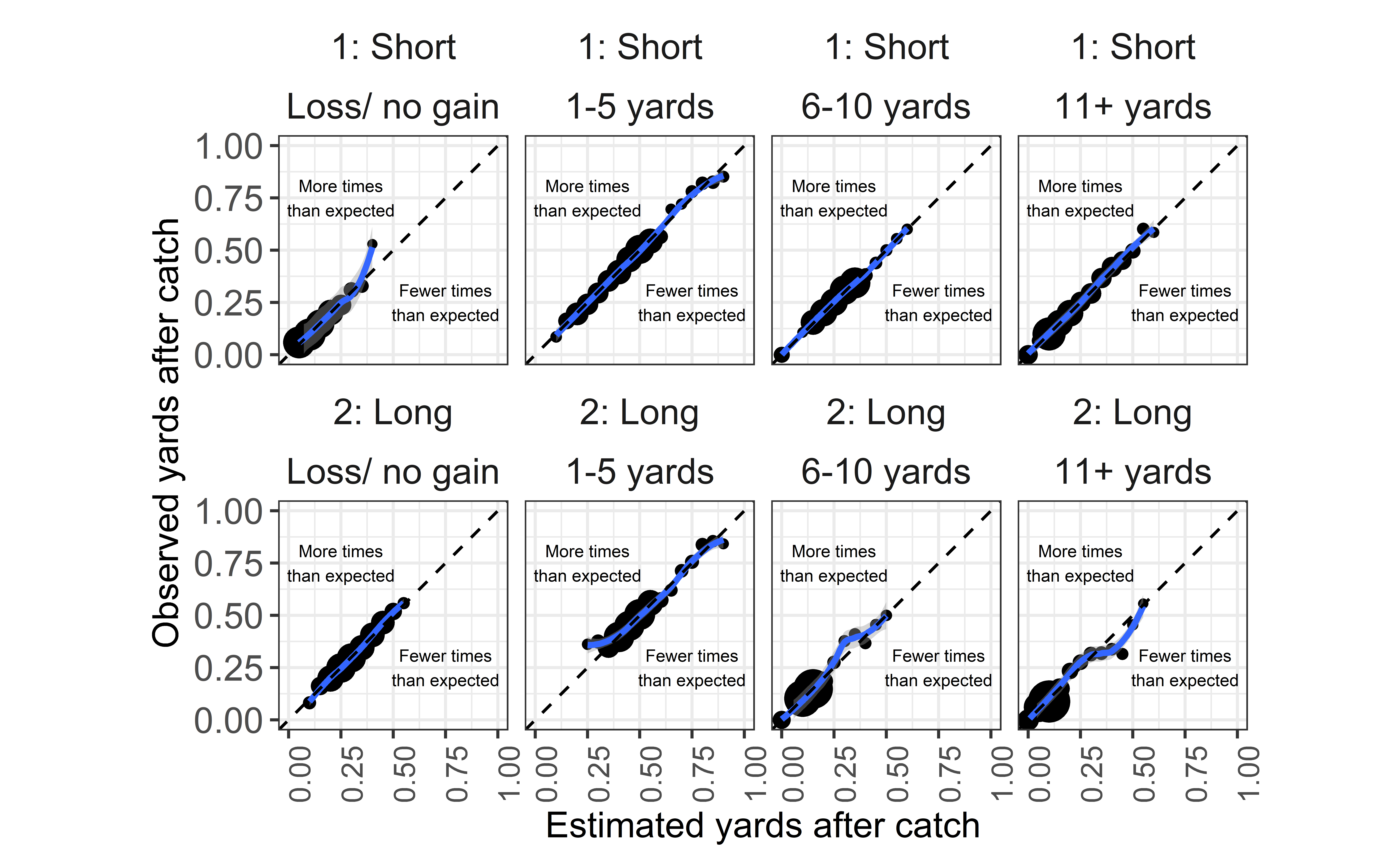
[1] 0.005xYAC Model Calibration Results
By now, the process should be familiar.
pbp_data <- readRDS(url("https://github.com/guga31bb/nflfastR-data/blob/master/models/cal_data.rds?raw=true"))
# pbp_data <- readRDS('../../nflfastR-data/models/cal_data.rds')

model_data <- pbp_data %>%
  make_model_mutations() %>%
  filter(
    season >= 2006, complete_pass == 1, !is.na(yards_after_catch),
    yards_after_catch >= -20, air_yards < yardline_100
  ) %>%
  dplyr::mutate(
    distance_to_goal = yardline_100 - air_yards,
    pass_middle = dplyr::if_else(pass_location == "middle", 1, 0),
    air_is_zero = dplyr::if_else(air_yards == 0, 1, 0),
    distance_to_sticks = air_yards - ydstogo,
    yards_after_catch = dplyr::case_when(
      yards_after_catch < -5 ~ -5,
      yards_after_catch > 70 ~ 70,
      TRUE ~ yards_after_catch
    ),
    label = yards_after_catch + 5
  ) %>%
  dplyr::filter(!is.na(air_yards) & air_yards >= -15 & air_yards < 70 & !is.na(pass_location)) %>%
  dplyr::select(
    season, label, air_yards, yardline_100, ydstogo, distance_to_goal,
    down1, down2, down3, down4, air_is_zero, pass_middle,
    era2, era3, era4, qb_hit, home,
    outdoors, retractable, dome, distance_to_sticks
  )


# nrounds = 500
nrounds <- 500
params <-
  list(
    booster = "gbtree",
    objective = "multi:softprob",
    eval_metric = c("mlogloss"),
    num_class = 76,
    eta = .025,
    gamma = 2,
    subsample = 0.8,
    colsample_bytree = 0.8,
    max_depth = 4,
    min_child_weight = 1
  )


cv_results <- map_dfr(2006:2019, function(x) {
  test_data <- model_data %>%
    filter(season == x) %>%
    select(-season)
  train_data <- model_data %>%
    filter(season != x) %>%
    select(-season)

  full_train <- xgboost::xgb.DMatrix(model.matrix(~ . + 0, data = train_data %>% select(-label)), label = train_data$label)
  xyac_model <- xgboost::xgboost(params = params, data = full_train, nrounds = nrounds, verbose = 2)

  preds <- as.data.frame(
    matrix(predict(xyac_model, as.matrix(test_data %>% select(-label))), ncol = 76, byrow = TRUE)
  )

  cv_data <- bind_cols(test_data, preds) %>%
    mutate(season = x)
  return(cv_data)
})
plot <- cv_results %>%
  select(label, air_yards, starts_with("V")) %>%
  mutate(
    loss = V1 + V2 + V3 + V4 + V5 + V6,
    short_gain = V7 + V8 + V9 + V10 + V11,
    med_gain = V12 + V13 + V14 + V15 + V16,
    long_gain = select(., V17:V76) %>% rowSums(),
    outcome = case_when(
      label <= 5 ~ "loss",
      between(label, 6, 10) ~ "short_gain",
      between(label, 11, 15) ~ "med_gain",
      label > 15 ~ "long_gain"
    ),
    distance = case_when(
      air_yards < 5 ~ "1: Short",
      air_yards >= 5 ~ "2: Long"
    )
  ) %>%
  select(outcome, distance, loss, short_gain, med_gain, long_gain) %>%
  pivot_longer(-c(outcome, distance), names_to = "type", values_to = "pred_prob") %>%
  mutate(bin_pred_prob = round(pred_prob / 0.05) * .05) %>%
  group_by(type, distance, bin_pred_prob) %>%
  mutate(correct = if_else(outcome == type, 1, 0)) %>%
  summarize(
    n_plays = n(),
    n_outcome = sum(correct),
    bin_actual_prob = n_outcome / n_plays
  )

ann_text <- data.frame(
  x = c(.25, 0.75), y = c(0.75, 0.25),
  lab = c("More times\nthan expected", "Fewer times\nthan expected")
)
plot %>%
  ungroup() %>%
  mutate(
    type = fct_relevel(
      type,
      "loss", "short_gain",
      "med_gain", "long_gain"
    ),
    type = fct_recode(type,
      "Loss/ no gain" = "loss",
      "1-5 yards" = "short_gain",
      "6-10 yards" = "med_gain",
      "11+ yards" = "long_gain"
    )
  ) %>%
  filter(n_plays > 15) %>%
  ggplot() +
  geom_point(aes(x = bin_pred_prob, y = bin_actual_prob, size = n_plays)) +
  geom_smooth(aes(x = bin_pred_prob, y = bin_actual_prob), method = "loess") +
  geom_abline(slope = 1, intercept = 0, color = "black", lty = 2) +
  coord_equal() +
  scale_x_continuous(limits = c(0, 1)) +
  scale_y_continuous(limits = c(0, 1)) +
  labs(
    size = "Number of plays",
    x = "Estimated yards after catch",
    y = "Observed yards after catch"
  ) +
  geom_text(data = ann_text, aes(x = x, y = y, label = lab), size = 2) +
  theme_bw() +
  theme(
    plot.title = element_text(hjust = 0.5),
    strip.background = element_blank(),
    strip.text = element_text(size = 12),
    axis.title = element_text(size = 12),
    axis.text.y = element_text(size = 12),
    axis.text.x = element_text(size = 10, angle = 90),
    legend.title = element_text(size = 12),
    legend.text = element_text(size = 12),
    legend.position = c(1.5, .05), legend.justification = c(1, 0)
  ) +
  facet_wrap(~ distance + type, ncol = 4)
Calibration error:
xyac_cv_cal_error <- plot %>%
  ungroup() %>%
  mutate(cal_diff = abs(bin_pred_prob - bin_actual_prob)) %>%
  group_by(distance) %>%
  summarize(
    weight_cal_error = weighted.mean(cal_diff, n_plays, na.rm = TRUE),
    n_outcome = sum(n_outcome, na.rm = TRUE)
  )

round(with(xyac_cv_cal_error, weighted.mean(weight_cal_error, n_outcome)), 4)
[1] 0.0058Expected Pass Model Calibration Results
By now, the process should be super familiar.
# model_data <- readRDS(url('https://github.com/guga31bb/nflfastR-data/blob/master/models/_dropback_model_data.rds?raw=true'))

model_data <- readRDS("_dropback_model_data.rds")

nrounds <- 1121
params <-
  list(
    booster = "gbtree",
    objective = "binary:logistic",
    eval_metric = c("error", "logloss"),
    eta = .015,
    gamma = 2,
    subsample = 0.8,
    colsample_bytree = 0.8,
    max_depth = 7,
    min_child_weight = 0.9,
    base_score = mean(model_data$label)
  )

cv_results <- map_dfr(2006:2019, function(x) {
  test_data <- model_data %>%
    filter(season == x) %>%
    select(-season)
  train_data <- model_data %>%
    filter(season != x) %>%
    select(-season)

  full_train <- xgboost::xgb.DMatrix(model.matrix(~ . + 0, data = train_data %>% select(-label)),
    label = train_data$label
  )
  xp_model <- xgboost::xgboost(params = params, data = full_train, nrounds = nrounds, verbose = 2)

  preds <- as.data.frame(
    matrix(predict(xp_model, as.matrix(test_data %>% select(-label))))
  ) %>%
    dplyr::rename(xp = V1)

  cv_data <- bind_cols(test_data, preds) %>% mutate(season = x)
  return(cv_data)
})

# TIME FOR BINNING
xp_cv_loso_calibration_results <- cv_results %>%
  # Create BINS for wp:
  mutate(
    bin_pred_prob = round(xp / 0.05) * .05,
    situation = case_when(
      down == 1 & ydstogo == 10 ~ "1st & 10",
      down == 2 ~ "2nd down",
      down == 3 ~ "3rd down",
      TRUE ~ "Other"
    )
  ) %>%
  # Group by both the qtr and bin_pred_prob:
  group_by(situation, bin_pred_prob) %>%
  # Calculate the calibration results:
  summarize(
    n_plays = n(),
    n_complete = length(which(label == 1)),
    bin_actual_prob = n_complete / n_plays
  )

ann_text <- data.frame(
  x = c(.25, 0.75), y = c(0.75, 0.25),
  lab = c("More times\nthan expected", "Fewer times\nthan expected")
)
Plot the results:
xp_cv_loso_calibration_results %>%
  ungroup() %>%
  mutate(situation = fct_relevel(
    situation,
    "1st & 10", "2nd down", "3rd down", "Other"
  )) %>%
  filter(n_plays > 10) %>%
  ggplot() +
  geom_point(aes(x = bin_pred_prob, y = bin_actual_prob, size = n_plays)) +
  geom_smooth(aes(x = bin_pred_prob, y = bin_actual_prob), method = "loess") +
  geom_abline(slope = 1, intercept = 0, color = "black", lty = 2) +
  coord_equal() +
  scale_x_continuous(limits = c(0, 1)) +
  scale_y_continuous(limits = c(0, 1)) +
  labs(
    size = "Number of plays",
    x = "Estimated dropback percentage",
    y = "Observed dropback percentage"
  ) +
  geom_text(data = ann_text, aes(x = x, y = y, label = lab), size = 3) +
  theme_bw() +
  theme(
    plot.title = element_text(hjust = 0.5),
    strip.background = element_blank(),
    strip.text = element_text(size = 12),
    axis.title = element_text(size = 12),
    axis.text.y = element_text(size = 12),
    axis.text.x = element_text(size = 10, angle = 90),
    legend.title = element_text(size = 12),
    legend.text = element_text(size = 12),
    legend.position = "bottom"
  ) +
  facet_wrap(~situation, ncol = 4)
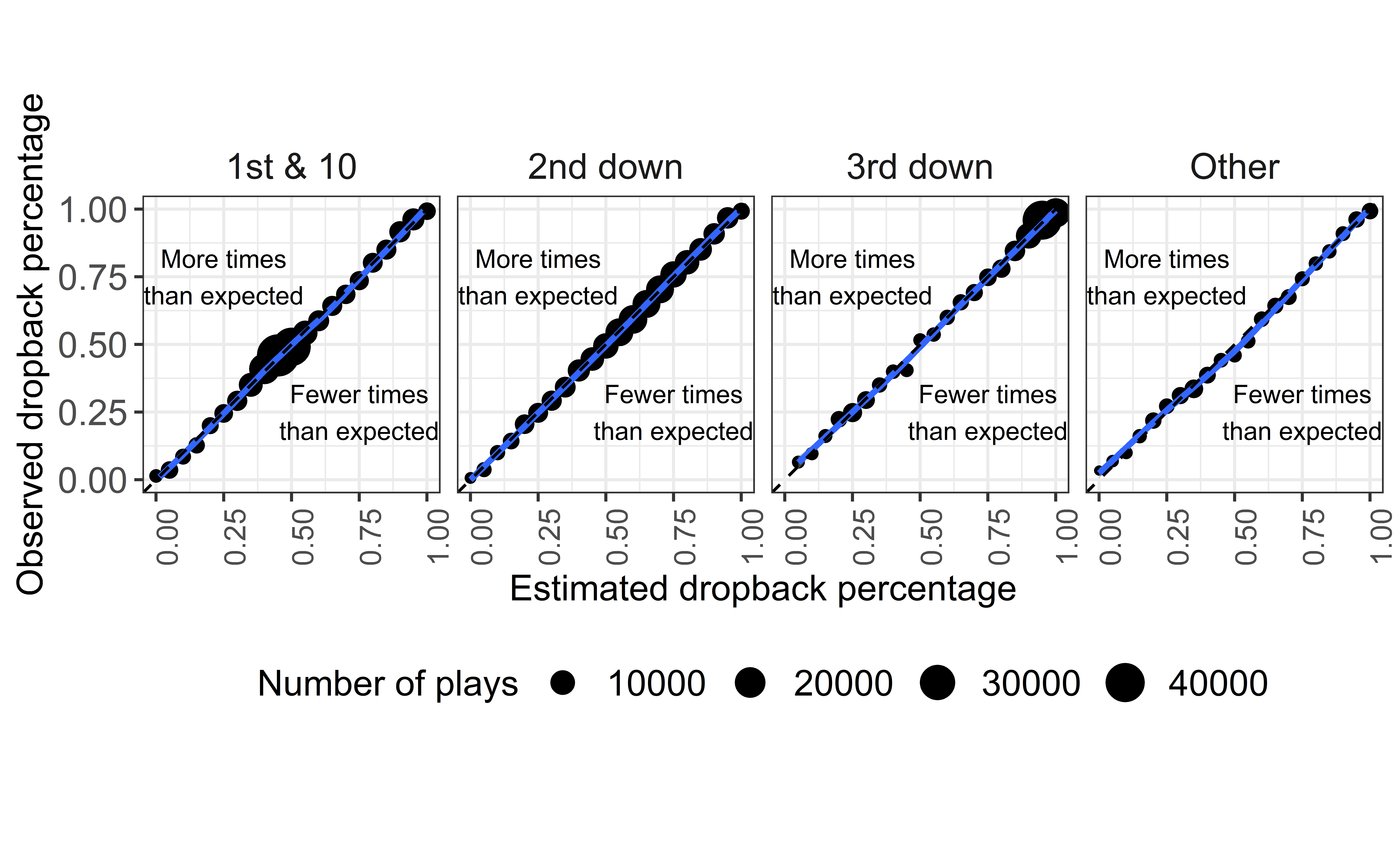
And get the calibration error:
xp_cv_cal_error <- xp_cv_loso_calibration_results %>%
  ungroup() %>%
  mutate(cal_diff = abs(bin_pred_prob - bin_actual_prob)) %>%
  group_by(situation) %>%
  summarize(
    weight_cal_error = weighted.mean(cal_diff, n_plays, na.rm = TRUE),
    n_complete = sum(n_complete, na.rm = TRUE)
  )

round(with(xp_cv_cal_error, weighted.mean(weight_cal_error, n_complete)), 4)
[1] 0.008