Open Source Football: Expected Turnovers for Quarterbacks

Anthony Gadaleta

Intro

Outside of actually scoring points, few events can swing an NFL game the way an interception or fumble can. Over the course of a season, if your quarterback is continuously giving the football away to the other team, your odds of a successful season are likely quite low.

With that said, all turnovers, and specifically QB turnovers, are not created equal. The goal of expected interceptions, expected fumbles and (by adding them together) expected turnovers is to measure how likely an incomplete pass or fumble is to be converted to an interception or lost fumble.¹

Load Packages, Get the Data


library(nflfastR)
library(tidyverse)
library(caret)
library(ggimage)
library(gt)

Download the latest play-by-play data for all plays from 2006-2019. We’ll be using 2006 as the start year because that’s the first year we have air yards data fully accessible.


seasons <- 2006:2019
pbp <- purrr::map_df(seasons, function(x) {
  readRDS(
    url(
      glue::glue("https://raw.githubusercontent.com/guga31bb/nflfastR-data/master/data/play_by_play_{x}.rds")
    )
  )
})

Download all NFL roster data from 1999-2019.


roster <- readRDS(url("https://raw.githubusercontent.com/guga31bb/nflfastR-data/master/roster-data/roster.rds"))

Expected Interceptions

We’ll start with building the model for expected interceptions. Our independent variables will be air yards, pass location, qb hits, number of pass defenders and season.

Start by creating an incompletions dataframe, which filters out all plays that do not result in incomplete passes or interceptions. Additionally, create the pass broken up (pbu) variable based on the number of pass defenders listed. The assumption being if more defenders are listed as defending a given pass, the more congested the throwing lane was.


incompletions <- pbp %>%
  filter(season_type == "REG" & season >= 2006 & (incomplete_pass == 1 | interception == 1)) %>%
  select(
    incomplete_pass, air_yards, pass_defense_1_player_id, pass_defense_2_player_id,
    season, posteam, interception, qb_hit, week, defteam, passer, posteam, pass_location, desc
  ) %>%
  mutate(
    pbu = case_when(
      !is.na(pass_defense_1_player_id) & !is.na(pass_defense_2_player_id) &
        (incomplete_pass == 1 | interception == 1) ~ 2,
      !is.na(pass_defense_1_player_id) & is.na(pass_defense_2_player_id) &
        (incomplete_pass == 1 | interception == 1) ~ 1,
      TRUE ~ 0
    ),
  )
incompletions$air_yards[is.na(incompletions$air_yards)] <- 0
incompletions$pass_location[is.na(incompletions$pass_location)] <- "None"

Split into training and testing dataframes. I used 2006-2016 to train the model and 2017-2019 to test. The split comes out to approximately 79% training, 21% testing.


int_train <- incompletions %>%
  filter(season < 2017) %>%
  select(-c(
    pass_defense_1_player_id, pass_defense_2_player_id, incomplete_pass, posteam, week, defteam,
    passer, posteam, desc
  )) %>%
  mutate(
    interception = if_else(interception == 1, "int", "no.int"),
  )

int_test <- incompletions %>%
  filter(season >= 2017)

Train the model using logistic regression, then add expected interceptions to the int_test dataframe.


fitControl <- trainControl(
  method = "repeatedcv",
  number = 10,
  repeats = 10,
  classProbs = TRUE,
  summaryFunction = twoClassSummary
)

set.seed(69) # nice
int_model <- train(interception ~ .,
  data = int_train,
  method = "glm", preProcess = c("scale", "center"),
  metric = "ROC", trControl = fitControl
)
int_model


Generalized Linear Model 

74261 samples
    5 predictor
    2 classes: 'int', 'no.int' 

Pre-processing: scaled (7), centered (7) 
Resampling: Cross-Validated (10 fold, repeated 10 times) 
Summary of sample sizes: 66835, 66835, 66835, 66835, 66834, 66834, ... 
Resampling results:

  ROC        Sens       Spec     
  0.9067668  0.1193285  0.9968662


int_test$exp_int <- predict(int_model, int_test, type = "prob")

Let’s take a look at the incompletions most likely have been intercepted from 2017-2019:


int_test %>%
  arrange(-exp_int) %>%
  select(desc, exp_int, passer, posteam, defteam, season, week) %>%
  head(5)


# A tibble: 5 x 7
  desc         exp_int$int $no.int passer posteam defteam season  week
  <chr>              <dbl>   <dbl> <chr>  <chr>   <chr>    <int> <int>
1 (:03) (Shot~       0.986  0.0141 D.Wat~ HOU     NE        2017     3
2 (:03) (Shot~       0.985  0.0153 J.All~ BUF     JAX       2018    12
3 (2:09) 73-C~       0.984  0.0158 M.Tru~ CHI     NO        2019     7
4 (2:41) 5-J.~       0.983  0.0167 J.Fla~ BAL     TEN       2017     9
5 (4:45) (Sho~       0.983  0.0175 M.Sta~ DET     NYG       2017     2

Expected Fumbles

Next up, we’ll build the expected fumbles model, using fumble forced vs not forced, fumble out of bounds, yards gained, sacks and aborted snaps as our independent variables.

Start by creating a fumbles dataframe, which includes all plays where the ball hits the turf, regardless of which team recovers.


fumbles <- pbp %>%
  filter(season_type == "REG", season >= 2006, fumble == 1) %>%
  select(
    fumble_forced, fumble_not_forced, fumble_out_of_bounds, fumble_lost, fumble, yards_gained, sack,
    aborted_play, season, posteam, week, defteam, fumbled_1_player_name, desc
  )

Splitting the same way as the incompletions, this time for an 80-20 train-test split.


fumble_train <- fumbles %>%
  filter(season < 2017) %>%
  select(-c(season, posteam, week, fumble, defteam, fumbled_1_player_name, desc)) %>%
  mutate(
    fumble_lost = if_else(fumble_lost == 1, "lost", "recovered")
  )
fumble_test <- fumbles %>%
  filter(season >= 2017)

Train the model using logistic regression (we can reuse the trControl from above) and then add expected fumbles to the fumble_test dataframe.


set.seed(69) # nice
fumble_model <- train(fumble_lost ~ .,
  data = fumble_train,
  method = "glm", preProcess = c("scale", "center"),
  trControl = fitControl, metric = "ROC"
)
fumble_model


Generalized Linear Model 

7642 samples
   6 predictor
   2 classes: 'lost', 'recovered' 

Pre-processing: scaled (6), centered (6) 
Resampling: Cross-Validated (10 fold, repeated 10 times) 
Summary of sample sizes: 6878, 6877, 6878, 6878, 6878, 6878, ... 
Resampling results:

  ROC        Sens       Spec     
  0.7115302  0.7990853  0.5359961


fumble_test$exp_fl <- predict(fumble_model, fumble_test, type = "prob")

Let’s take a look at the fumbles most likely to have been lost from 2017-2019:


fumble_test %>%
  arrange(-exp_fl) %>%
  select(desc, exp_fl, fumbled_1_player_name, posteam, defteam, season, week) %>%
  head(5)


# A tibble: 5 x 7
  desc  exp_fl$lost $recovered fumbled_1_playe~ posteam defteam season
  <chr>       <dbl>      <dbl> <chr>            <chr>   <chr>    <int>
1 (:01~       0.852      0.148 T.Cohen          CHI     GB        2019
2 (:05~       0.834      0.166 J.Witten         DAL     GB        2017
3 (10:~       0.834      0.166 J.Jones          KC      LAC       2018
4 (:02~       0.834      0.166 J.Edelman        NE      MIA       2019
5 (:04~       0.824      0.176 J.Crowder        WAS     KC        2017
# ... with 1 more variable: week <int>

Predictive Power?

Now it’s time to see if these new stats are actually useful for predicting future turnovers.

First, modify roster names to allow us to use merge roster data with the dataframes we created above.


roster$name <- paste0(substr(roster$teamPlayers.firstName, 1, 1), ".", roster$teamPlayers.lastName)

Merge roster data and group by passer and season to get total interceptions and expected interceptions and then total fumbles lost and expected fumbles lost for each passer in each season.


xInt <- int_test %>%
  filter(!is.na(passer)) %>%
  left_join(roster[, c(
    "team.season", "name", "teamPlayers.position", "team.abbr",
    "teamPlayers.headshot_url"
  )],
  by = c("passer" = "name", "season" = "team.season", "posteam" = "team.abbr")
  ) %>%
  rename(
    position = teamPlayers.position,
    player = passer,
  ) %>%
  filter(position == "QB") %>%
  group_by(player, posteam, season, teamPlayers.headshot_url) %>%
  summarise(Interceptions = sum(interception), xInt = sum(exp_int$int)) %>%
  mutate(diff = Interceptions - xInt)

xFmb <- fumble_test %>%
  filter(!is.na(fumbled_1_player_name)) %>%
  left_join(roster[, c(
    "team.season", "name", "teamPlayers.position", "team.abbr",
    "teamPlayers.headshot_url"
  )],
  by = c("fumbled_1_player_name" = "name", "season" = "team.season", "posteam" = "team.abbr")
  ) %>%
  rename(
    position = teamPlayers.position,
    player = fumbled_1_player_name,
  ) %>%
  filter(position == "QB") %>%
  group_by(player, posteam, season, teamPlayers.headshot_url) %>%
  summarise(Fumbles_Lost = sum(fumble_lost), xFmb = sum(exp_fl$lost)) %>%
  mutate(diff = Fumbles_Lost - xFmb)

Find total dropbacks, epa per dropback and success rate on dropbacks for each passer. The latter two stats really aren’t necessary, but I thought it could be useful to show how well certain quarterbacks performed overall.


dropbacks <- pbp %>%
  filter(season_type == "REG" & season > 2016 & !is.na(passer)) %>%
  group_by(passer, season) %>%
  summarise(dropbacks = n(), epa = mean(epa, na.rm = TRUE), sr = mean(success, na.rm = TRUE))

Merge the dropbacks dataframe with the xInt and xFmb dataframes. Then calc total turnovers, expected turnovers, turnovers per dropback, interceptions per dropback, differences between all of the actual and expected stats and the next season’s turnovers, interceptions and fumbles.


xTO <- dropbacks %>%
  inner_join(xInt, by = c("passer" = "player", "season")) %>%
  left_join(xFmb, by = c("passer" = "player", "posteam", "season", "teamPlayers.headshot_url"))

xTO$Fumbles_Lost[is.na(xTO$Fumbles_Lost)] <- 0
xTO$xFmb[is.na(xTO$xFmb)] <- 0
xTO$diff.y[is.na(xTO$diff.y)] <- 0

xTO <- xTO %>%
  mutate(
    Turnovers = Interceptions + Fumbles_Lost,
    xTO = xInt + xFmb,
    diff = diff.x + diff.y,
    to_pct = Turnovers / dropbacks,
    int_pct = Interceptions / dropbacks,
    xto_pct = xTO / dropbacks,
    xint_pct = xInt / dropbacks,
    to_pct_diff = xto_pct - to_pct,
    int_pct_diff = xint_pct - int_pct,
  ) %>%
  filter(dropbacks >= 250) %>%
  group_by(passer) %>%
  mutate(
    next_to = lead(Turnovers, 1),
    next_int = lead(Interceptions, 1),
    next_fmb = lead(Fumbles_Lost, 1),
    next_db = lead(dropbacks, 1)
  )

Finally, let’s evaluate how predictive our new expected statistics are compared to their standard counterparts.


[1] "R2 of current TOs to next season's TOs: 0.187481148618913"


[1] "R2 of current xTO to next season's TOs: 0.118063100859092"


[1] "R2 of current Ints to next season's Ints: 0.178815133484698"


[1] "R2 of current xInts to next season's Ints: 0.144854426175095"


[1] "R2 of current Fumbles to next season's Fumbles: 0.204064081434686"


[1] "R2 of current xFmb to next season's Fumbles: 0.106391377897902"

As we can see, the “regular” stats outperform all of the expected turnover statistics. But what if we look at these as rate stats per dropback?


[1] "R2 of current TOs per dropback to next season's TOs per dropback: 0.259161533025725"


[1] "R2 of current xTOs per dropback to next season's TOs per dropback: 0.315618037803437"


[1] "R2 of current Ints per dropback to next season's Ints per dropback: 0.211910004427118"


[1] "R2 of current xInts per dropback to next season's Ints per dropback: 0.297221826811028"

Now we’ve got some winners! We can predict next season’s turnovers and interceptions per dropback more effectively using xTOs and xInts per dropback than we can using the ordinary rate stats.

Visuals

Finally, we can plot the results to help us visualize who is most likely to turn the ball over at a higher or lower rate next season.


ggplot(subset(xTO, season == 2019), aes(x = Turnovers / dropbacks, y = xTO / dropbacks)) +
  geom_image(aes(image = teamPlayers.headshot_url), size = 0.05, asp = 16 / 9) +
  labs(
    title = "QB Turnovers 2019",
    subtitle = "Regular Season | Min. 250 Dropbacks",
    x = "Actual Turnovers per Dropback",
    y = "Expected Turnovers per Dropback",
    caption = "@AG_8 | Data: @nflfastR"
  ) +
  theme_bw() +
  theme(
    aspect.ratio = 9 / 16,
    plot.title = element_text(size = 12, hjust = 0.5, face = "bold"),
    plot.subtitle = element_text(size = 10, hjust = 0.5),
  ) +
  geom_abline(slope = 1, intercept = 0)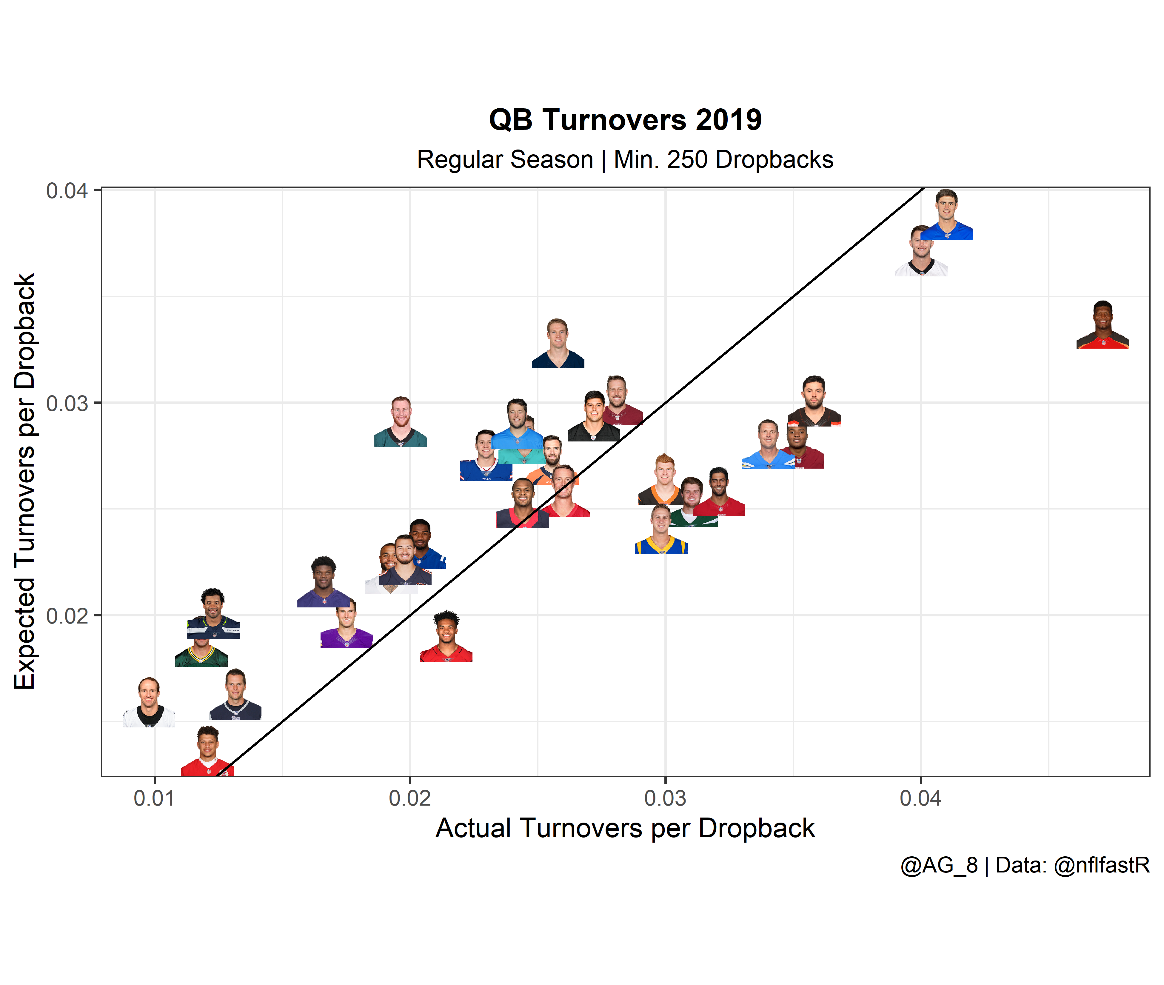


ggplot(subset(xTO, season == 2019), aes(x = Interceptions / dropbacks, y = xInt / dropbacks)) +
  geom_image(aes(image = teamPlayers.headshot_url), size = 0.05, asp = 16 / 9) +
  labs(
    title = "QB Interceptions 2019",
    subtitle = "Regular Season | Min. 250 Dropbacks",
    x = "Actual Interceptions per Dropback",
    y = "Expected Interceptions per Dropback",
    caption = "@AG_8 | Data: @nflfastR"
  ) +
  theme_bw() +
  theme(
    aspect.ratio = 9 / 16,
    plot.title = element_text(size = 12, hjust = 0.5, face = "bold"),
    plot.subtitle = element_text(size = 10, hjust = 0.5),
  ) +
  geom_abline(slope = 1, intercept = 0)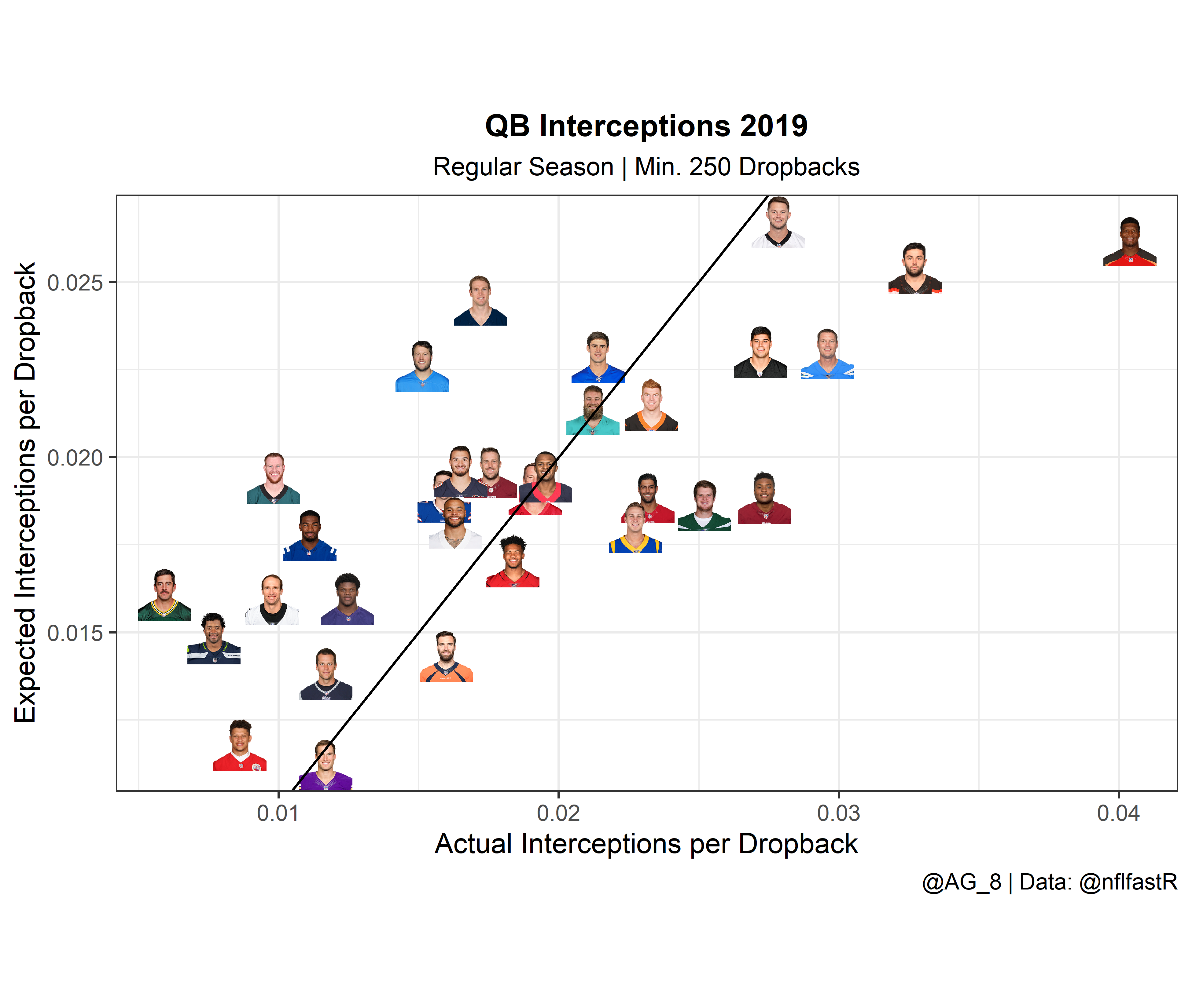

Lastly, we’ll use the gt package to make a really cool looking table of the 2019 data.


xTO %>%
  ungroup() %>%
  filter(season == 2019) %>%
  select(c(passer, posteam, dropbacks, to_pct, xto_pct, to_pct_diff, int_pct, xint_pct, int_pct_diff)) %>%
  mutate(
    to_pct_diff = to_pct_diff * 100,
    int_pct_diff = int_pct_diff * 100
  ) %>%
  gt() %>%
  tab_header(
    title = "Expected QB Turnovers",
    subtitle = "Regular Season 2019 | Min. 250 Dropbacks"
  ) %>%
  cols_label(
    passer = "QB",
    posteam = "Team",
    dropbacks = "Dropbacks",
    to_pct = "TOs per Dropback",
    xto_pct = "xTOs per Dropback",
    to_pct_diff = "xTOs/DB - TOs/DB",
    int_pct = "Ints per Dropback",
    xint_pct = "xInts per Dropback",
    int_pct_diff = "xInts/DB - Ints/DB"
  ) %>%
  fmt_number(
    columns = c("to_pct", "xto_pct", "to_pct_diff", "int_pct", "xint_pct", "int_pct_diff"),
    decimals = 2
  ) %>%
  fmt_percent(
    columns = c("to_pct", "xto_pct", "int_pct", "xint_pct")
  ) %>%
  tab_source_note("@AG_8 | Data: @nflfastR") %>%
  data_color(
    columns = c("to_pct", "xto_pct", "to_pct_diff", "int_pct", "xint_pct", "int_pct_diff"),
    colors = scales::col_numeric(palette = "Reds", domain = NULL)
  ) %>%
  cols_align(align = "center") %>%
  cols_width(
    everything() ~ px(90)
  )

Expected QB Turnovers
Regular Season 2019 \| Min. 250 Dropbacks
QB	Team	Dropbacks	TOs per Dropback	xTOs per Dropback	xTOs/DB - TOs/DB	Ints per Dropback	xInts per Dropback	xInts/DB - Ints/DB
A.Dalton	CIN	601	3.00%	2.64%	−0.35	2.33%	2.15%	−0.18
A.Rodgers	GB	677	1.18%	1.88%	0.70	0.59%	1.61%	1.02
B.Mayfield	CLE	642	3.58%	3.01%	−0.57	3.27%	2.54%	−0.73
C.Keenum	WAS	285	2.81%	3.02%	0.21	1.75%	1.96%	0.21
C.Wentz	PHI	714	1.96%	2.92%	0.96	0.98%	1.94%	0.96
D.Brees	NO	410	0.98%	1.60%	0.62	0.98%	1.60%	0.62
D.Haskins	WAS	256	3.52%	2.81%	−0.70	2.73%	1.88%	−0.85
D.Jones	NYG	561	4.10%	3.89%	−0.21	2.14%	2.29%	0.15
D.Prescott	DAL	675	1.93%	2.22%	0.30	1.63%	1.81%	0.19
D.Watson	HOU	615	2.44%	2.53%	0.09	1.95%	1.95%	−0.01
J.Allen	BUF	566	2.30%	2.75%	0.46	1.59%	1.89%	0.30
J.Brissett	IND	540	2.04%	2.34%	0.30	1.11%	1.78%	0.67
J.Flacco	DEN	313	2.56%	2.74%	0.18	1.60%	1.43%	−0.16
J.Garoppolo	SF	561	3.21%	2.59%	−0.62	2.32%	1.89%	−0.43
J.Goff	LA	704	2.98%	2.41%	−0.57	2.27%	1.80%	−0.47
J.Winston	TB	743	4.71%	3.38%	−1.33	4.04%	2.62%	−1.42
K.Allen	CAR	575	4.00%	3.72%	−0.28	2.78%	2.67%	−0.11
K.Cousins	MIN	514	1.75%	1.97%	0.22	1.17%	1.12%	−0.04
K.Murray	ARI	654	2.14%	1.90%	−0.24	1.83%	1.70%	−0.13
L.Jackson	BAL	482	1.66%	2.16%	0.50	1.24%	1.60%	0.35
M.Rudolph	PIT	331	2.72%	2.94%	0.22	2.72%	2.30%	−0.42
M.Ryan	ATL	731	2.60%	2.59%	−0.01	1.92%	1.91%	−0.00
M.Stafford	DET	331	2.42%	2.91%	0.49	1.51%	2.26%	0.75
M.Trubisky	CHI	606	1.98%	2.27%	0.29	1.65%	1.96%	0.31
P.Mahomes	KC	581	1.20%	1.37%	0.16	0.86%	1.18%	0.32
P.Rivers	LAC	676	3.40%	2.81%	−0.59	2.96%	2.30%	−0.66
R.Fitzpatrick	MIA	613	2.45%	2.84%	0.39	2.12%	2.14%	0.02
R.Tannehill	TEN	349	2.58%	3.29%	0.71	1.72%	2.45%	0.73
R.Wilson	SEA	651	1.23%	2.01%	0.78	0.77%	1.48%	0.72
S.Darnold	NYJ	516	3.10%	2.54%	−0.56	2.52%	1.86%	−0.65
T.Brady	NE	685	1.31%	1.63%	0.32	1.17%	1.38%	0.21
@AG_8 \| Data: @nflfastR

Conclusion

Based on the table and plots above, we can see that Jameis had, by far, the largest difference between expected and actual turnovers. This really isn’t much of a shock since you of course need some bad luck to have as high of a turnover rate as he did.

Additionally, I found it interesting that although Rodgers and Wentz were two of “luckiest” with turnovers from last year, if they regress to their xTO and xInt numbers they would still be average or maybe even slightly above average, just in terms of turnovers.

Finally, although Daniel Jones and Kyle Allen were terrible in terms of hanging onto the rock last season, there isn’t a ton of hope for improvement for either. Both had xTO rates just slightly below their actual TO rates.

Without tracking data, it really doesn’t make sense to calculate the likelihood of an interception or fumble on all plays.↩

Expected Turnovers for Quarterbacks

Table of Contents