Table of Contents
Part 0: Background and summary
Elo is a ranking and prediction framework that 538 has successfully applied to the NFL. Because QB performance plays such a strong role in overall team performance, 538’s Elo framework models QB contributions separately before adding them back to the overall team grade.
These QB rankings significantly improve the overall predictive power of the framework, making them a fairly accurate measure of a QB’s value. Every 25 points of Elo are equivalent to roughly 1 point of expected game margin. For instance, a QB with an Elo of 100 would be worth roughly 4 points more per game than a replacement level QB.
Measuring the cumulative Elo added by a QB over the course of their career is akin to measuring the total points added above a replacement level player. In this post, QB Elo values are pulled from 538 and normalized by era, allowing for an interesting comparison of QB careers throughout the history of the NFL. As QB rankings can be a touchy subject, it is worth noting that these rankings are just one quantitative view of a QBs overall performance.
Part 1: Importing and cleaning data
First, import packages:
import pandas as pd
import numpy
import requests
import seaborn as sns
import matplotlib.pyplot as plt
Next, pull Elo data from 538 and load it into a pandas data frame:
data_link = 'https://projects.fivethirtyeight.com/nfl-api/nfl_elo.csv'
data_df = pd.read_csv(data_link)
We only want data with QB grades, and we’ll exclude playoffs:
data_df = data_df[(~numpy.isnan(data_df['qbelo1_pre'])) & (~numpy.isnan(data_df['qbelo2_pre']))]
data_df = data_df[data_df['playoff'].isna()]
Elo game data comes with game dates, not weeks:
data_df['date'].sample(5)
12007    2003-09-07
12393    2004-11-07
9108     1991-10-20
4180     1968-09-15
3363     1963-09-15
Name: date, dtype: object
Which we’ll want to convert to weeks to make them easier to group:
## create a datetime series from the date ##
data_df['date_time'] = pd.to_datetime(data_df['date'])

## mondays are new weeks, so subtract a day and then trunc to get an NFL week ##
data_df['date_time'] = data_df['date_time'] - pd.Timedelta(days=1)
data_df['week_of'] = data_df['date_time'].dt.week
Next, separate Home and Away data and merge it into a single flat file, filtering out unnecessary fields and renaming columns in the process:
## create a flat file ##
home_data_df = data_df.copy()[[
    'season',
    'week_of',
    'qb1',
    'qb1_value_post',
    'score1',
    'score2'
]].rename(columns={
    'qb1' : 'qb_name',
    'qb1_value_post' : 'qb_elo_value',
    'score1' : 'points_for',
    'score2' : 'points_against',
})

away_data_df = data_df.copy()[[
    'season',
    'week_of',
    'qb2',
    'qb2_value_post',
    'score2',
    'score1'
]].rename(columns={
    'qb2' : 'qb_name',
    'qb2_value_post' : 'qb_elo_value',
    'score2' : 'points_for',
    'score1' : 'points_against',
})

flat_df = pd.concat([home_data_df,away_data_df])
flat_df = flat_df.sort_values(by=['season','week_of'])
This yields a data frame with individual QB games:
flat_df.sample(5)
       season  week_of  ... points_for  points_against
11821    2002       41  ...         10              17
2500     1954       44  ...         30               6
5913     1977       38  ...         30              27
12046    2003       38  ...         12              13
5502     1975       38  ...         14              42

[5 rows x 6 columns]
Note that the above data are Elo values. To convert Elo values to Elo, you’d need to multiply by 3.3 per 538’s methodology. Add some addition stats:
flat_df['point_margin'] = flat_df['points_for'] - flat_df['points_against']
flat_df['win'] = numpy.where(flat_df['point_margin'] > 0,1,0)
Part 2: Adjusting for era
538’s QB ratings are based on stats that have increased overtime alongside improved QB play. This can be seen by looking at the median QB Elo value overtime:
## calculate median QB values by season week ##
median_df = flat_df.groupby(['season','week_of']).agg(
    qb_elo_value_median = ('qb_elo_value', 'median'),
    qb_elo_value_min = ('qb_elo_value', 'min'),
    qb_elo_value_max = ('qb_elo_value', 'max')
).reset_index()

## plot ##
median_line = median_df['qb_elo_value_median'].plot.line()
plt.show()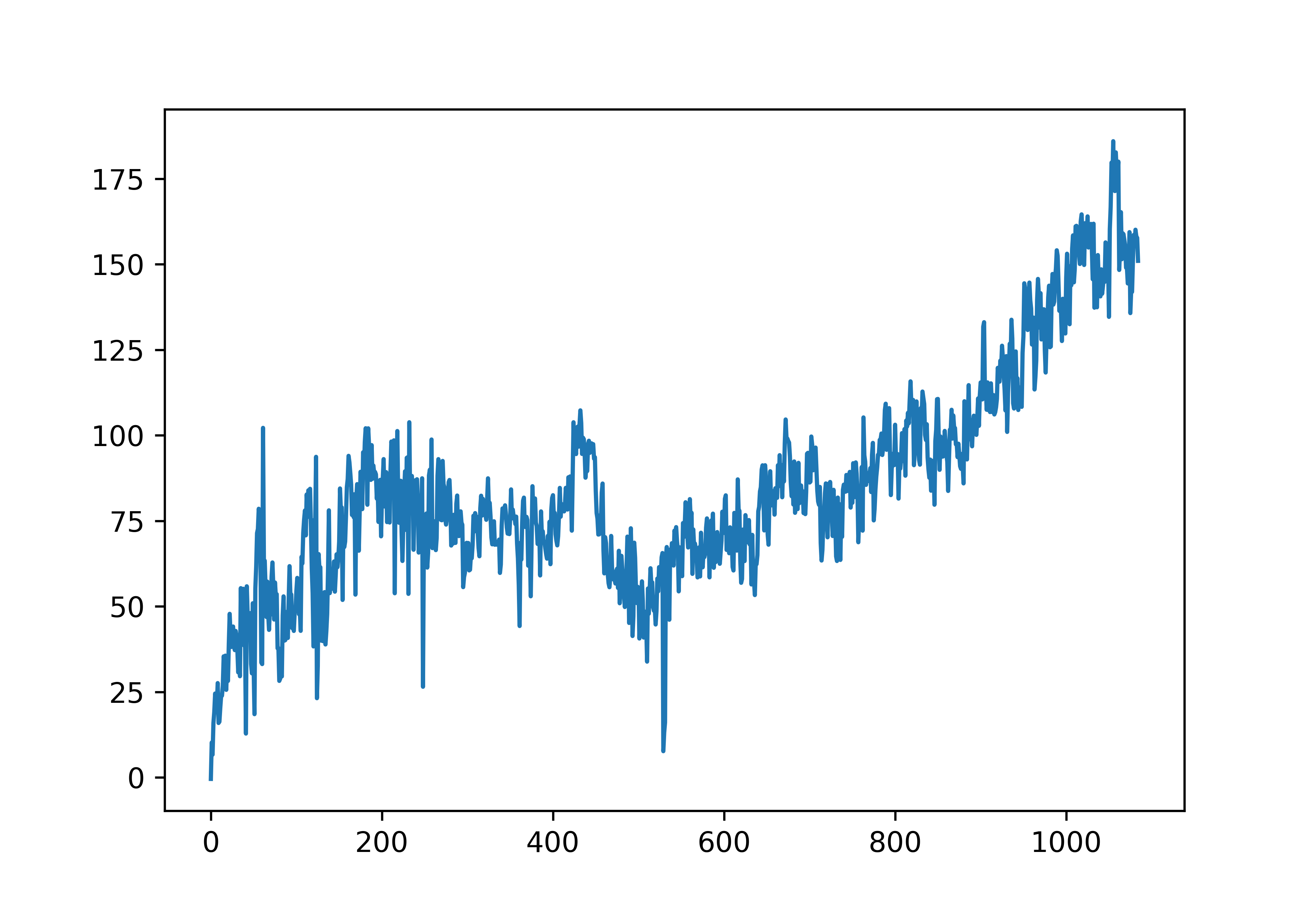
To make 538’s Elo values comparable across era, this stat inflation needs to be removed:
## add weekly median to flat file ##
flat_df = pd.merge(
    flat_df,
    median_df,
    on=['season','week_of'],
    how='left'
)

## calculate an adjusted stat that removes the median
flat_df['qb_elo_value_era_adjusted'] = flat_df['qb_elo_value'] - flat_df['qb_elo_value_median']
Part 3: Adding stats and compiling careers
To compare quarterbacks, we’ll need to aggregate all of their QB values, but first, some additional stats can be added to make the ultimate comparisons more interesting. Namely, Elo ranking relative to other starters at a point in time, total starts, and win percentages:
## add weekly ranking ##
flat_df['qb_rank'] = flat_df.groupby(['season','week_of'])['qb_elo_value'].rank(method='max', ascending=False)
flat_df['top_1_qb'] = numpy.where(flat_df['qb_rank']<=1, 1,0)
flat_df['top_3_qb'] = numpy.where(flat_df['qb_rank']<=3, 1,0)
flat_df['top_5_qb'] = numpy.where(flat_df['qb_rank']<=5, 1,0)

## add cumulative count ##
flat_df['game_number'] = flat_df.groupby(['qb_name']).cumcount() + 1
flat_df['cumulative_era_adjusted_value'] = flat_df.groupby('qb_name')['qb_elo_value_era_adjusted'].transform(pd.Series.cumsum)
flat_df['cumulative_wins'] = flat_df.groupby('qb_name')['win'].transform(pd.Series.cumsum)
flat_df['cumulative_best_starter'] = flat_df.groupby('qb_name')['top_1_qb'].transform(pd.Series.cumsum)
flat_df['cumulative_top_3_starts'] = flat_df.groupby('qb_name')['top_3_qb'].transform(pd.Series.cumsum)
flat_df['cumulative_top_5_starts'] = flat_df.groupby('qb_name')['top_5_qb'].transform(pd.Series.cumsum)
After adding stats, compile at the QB level to get a look at their career:
## aggregate ##
agg_df = flat_df.groupby('qb_name').agg(
    total_starts = ('game_number', 'max'),
    cumulative_era_adjusted_elo_value = ('qb_elo_value_era_adjusted', 'sum'),
    winning_percentage = ('win', 'mean'),
    pct_of_starts_as_best_qb = ('top_1_qb', 'mean'),
    pct_of_starts_as_top3_qb = ('top_3_qb', 'mean'),
    pct_of_starts_as_top5_qb = ('top_5_qb', 'mean')
).reset_index()

agg_df['average_era_adjusted_elo_value'] = agg_df['cumulative_era_adjusted_elo_value'] / agg_df['total_starts']
Sort by total Elo value to see the era adjusted rankings:
## sort ##
agg_df = agg_df.sort_values(by=['cumulative_era_adjusted_elo_value'],ascending=[False])[[
    'qb_name',
    'total_starts',
    'cumulative_era_adjusted_elo_value',
    'average_era_adjusted_elo_value',
    'winning_percentage',
    'pct_of_starts_as_best_qb',
    'pct_of_starts_as_top3_qb',
    'pct_of_starts_as_top5_qb'
]]

agg_df[['qb_name','total_starts','cumulative_era_adjusted_elo_value']].head(15)
            qb_name  total_starts  cumulative_era_adjusted_elo_value
493  Peyton Manning           265                       26065.054253
204      Drew Brees           274                       23763.826759
616       Tom Brady           283                       19225.832143
146      Dan Marino           240                       17160.155283
226  Fran Tarkenton           239                       14498.753253
338     Joe Montana           164                       14043.230167
73      Brett Favre           298                       12764.784141
588     Steve Young           143                       12689.178178
4     Aaron Rodgers           174                       12132.510866
364   Johnny Unitas           185                        9796.247620
144       Dan Fouts           171                        9767.284528
441       Matt Ryan           189                        8398.344958
380    Ken Anderson           172                        7866.688036
495   Philip Rivers           224                        7385.531378
347      John Elway           231                        7250.838144
Part 4: Graphing careers
Though simple, era adjusted QB Elo appears to provide a fairly good ranking of QBs across era. One interesting way to leverage this measure further is by comparing cumulative QB Elo gained over the course of a QB’s career.
Create a function for graphing career Elo based on a list of QBs:
def create_qb_chart(qbs_to_plot):
    ## plot career cumulative Elo value based on a list of QBs ##
    ## make a copy of the flat file ##
    chart_df = flat_df.copy()
    ## filter to just relevant fields ##
    chart_df = chart_df[[
        'qb_name',
        'game_number',
        'cumulative_era_adjusted_value'
    ]]
    ## create sub selection of QBs
    chart_df = chart_df[numpy.isin(
        chart_df['qb_name'],
        qbs_to_plot
    )]
    ## set up plot ##
    sns.lineplot(
        'game_number',
        'cumulative_era_adjusted_value',
        hue='qb_name',
        ci=None,
        palette='RdPu',
        data=chart_df
    )
    sns.despine()
    ## set axis titles and sizes ##
    plt.xlabel('Games Played', labelpad=10, fontsize='small', weight='bold')
    plt.ylabel('Cumulative Elo Value Added', labelpad=10, fontsize='small', weight='bold')
    plt.rc('xtick',labelsize='x-small')
    plt.rc('ytick',labelsize='x-small')
    ## define plot ranges, leaving a little room for padding ##
    xmin = 0
    xmax = chart_df['game_number'].max() * 1.2
    ymin = chart_df['cumulative_era_adjusted_value'].min() * 1.15
    ymax = chart_df['cumulative_era_adjusted_value'].max() * 1.15
    plt.xlim(xmin,xmax)
    plt.ylim(ymin,ymax)
    ## add darker axis ##
    plt.axhline(y = ymin, color = 'black', linewidth = 1.75)
    plt.axvline(x = xmin, color = 'black', linewidth = 1.75)
    ## and a line at zero
    plt.axhline(y = 0, color = 'black', linewidth = 0.75)
    ## add labels at the end of each line ##
    for i in qbs_to_plot:
        plt.text(
            x = chart_df[chart_df['qb_name'] == i]['game_number'].iloc[-1] + 1,
            y = chart_df[chart_df['qb_name'] == i]['cumulative_era_adjusted_value'].iloc[-1] + 5,
            s = i,
            weight = 'bold',
            fontsize = 'small',
            backgroundcolor = '#ffffff'
        )
    ## remove legend ##
    plt.legend([],[], frameon=False)
    plt.tight_layout()
Make your comparisons…
Manning, Brady, and Brees:
qb_list = ['Tom Brady', 'Peyton Manning','Drew Brees']
create_qb_chart(qb_list)
plt.show()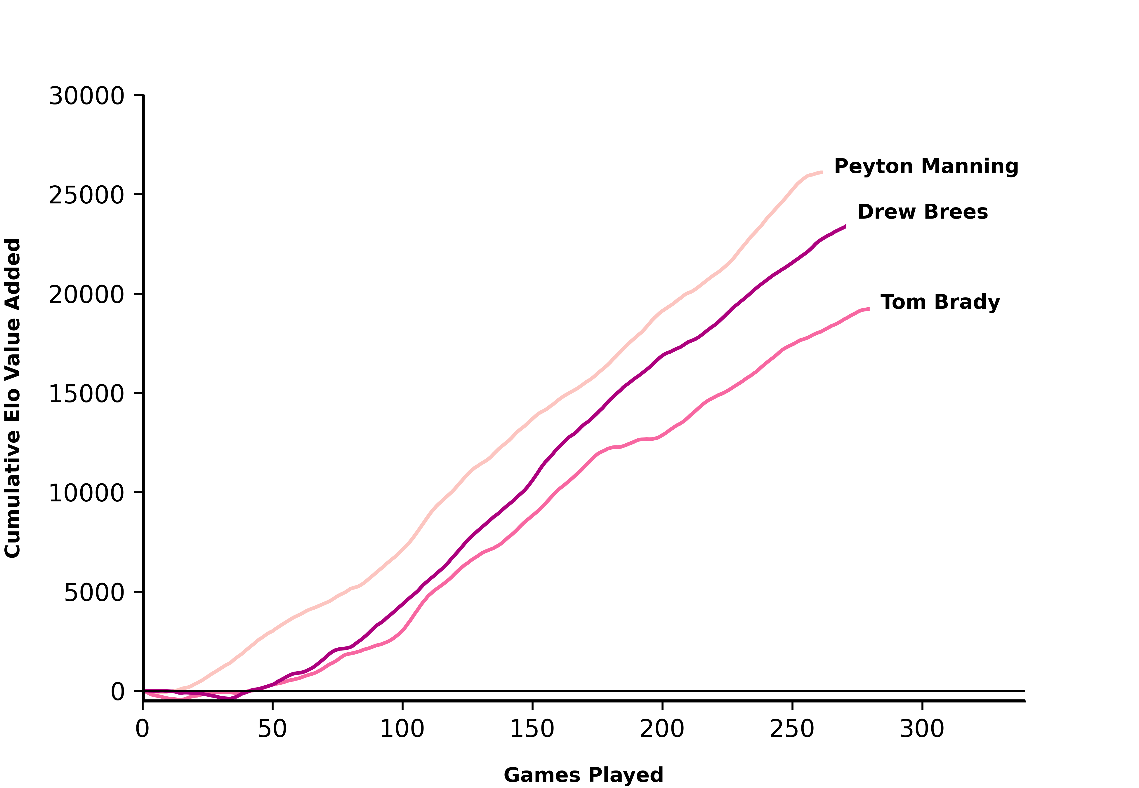
Romo > Dak > Aikman?:
qb_list = ['Tony Romo', 'Troy Aikman', 'Dak Prescott']
create_qb_chart(qb_list)
plt.show()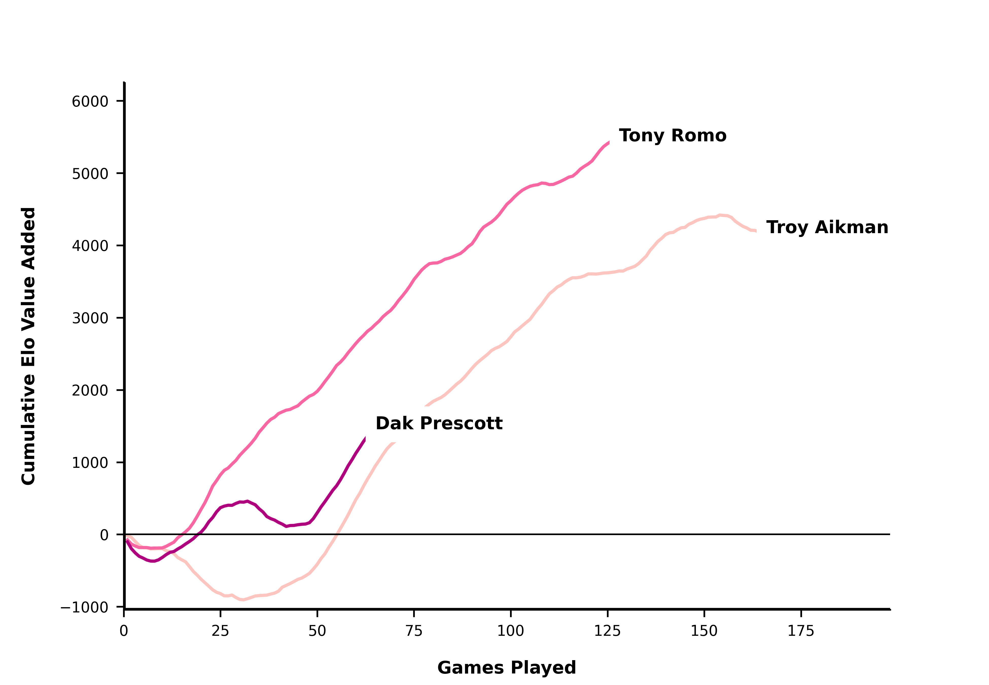
JaMarcus Russell, it could have been worse:
qb_list = ['JaMarcus Russell', 'Johnny Manziel', 'Ryan Leaf']
create_qb_chart(qb_list)
plt.show()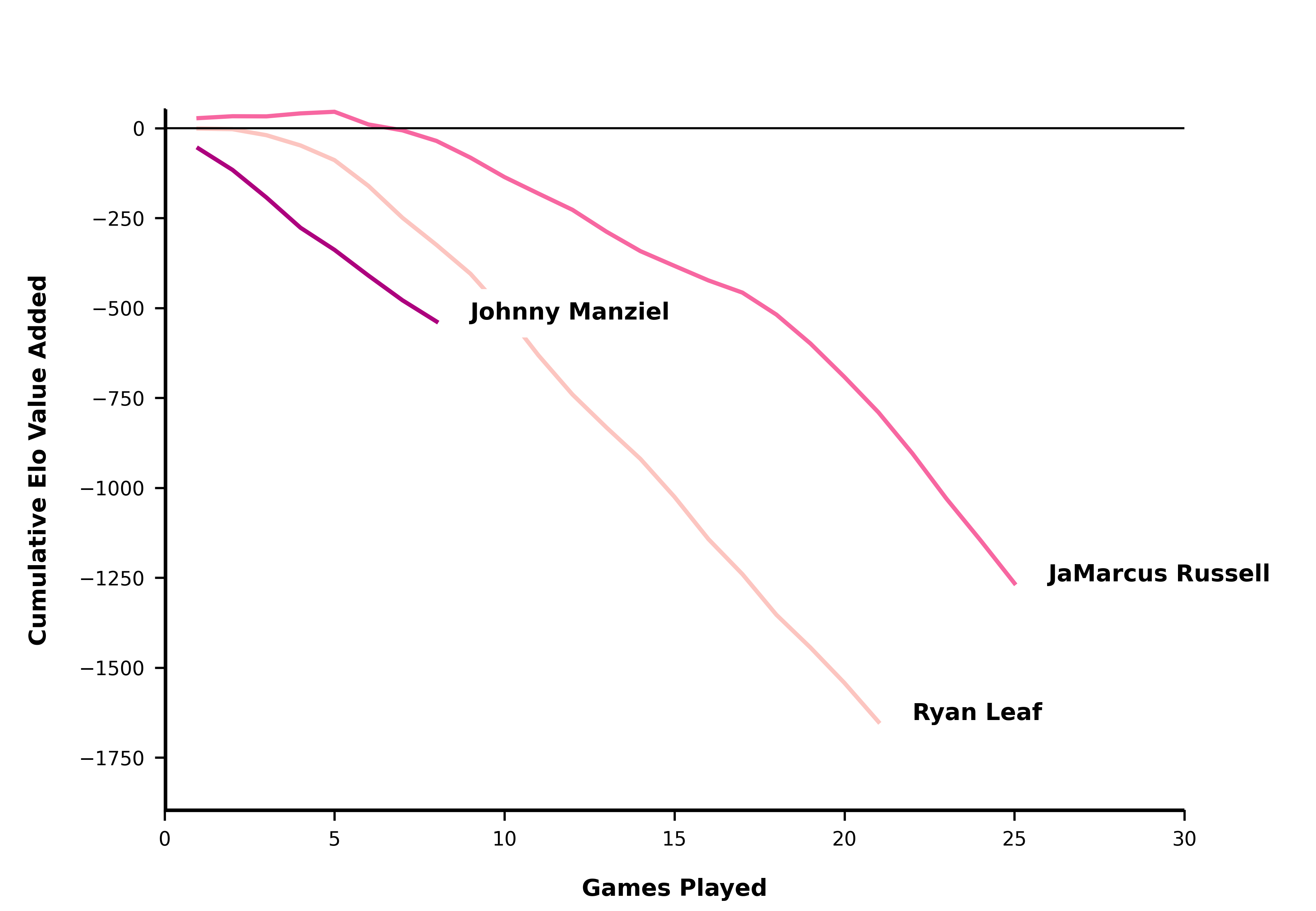
Maybe Leaf just needed more time and a better defense:
qb_list = ['Ryan Leaf', 'Trent Dilfer']
create_qb_chart(qb_list)
plt.show()
Mahomes, off to one of the best starts ever:
qb_list = ['Patrick Mahomes', 'Aaron Rodgers', 'Dan Marino']
create_qb_chart(qb_list)
plt.show()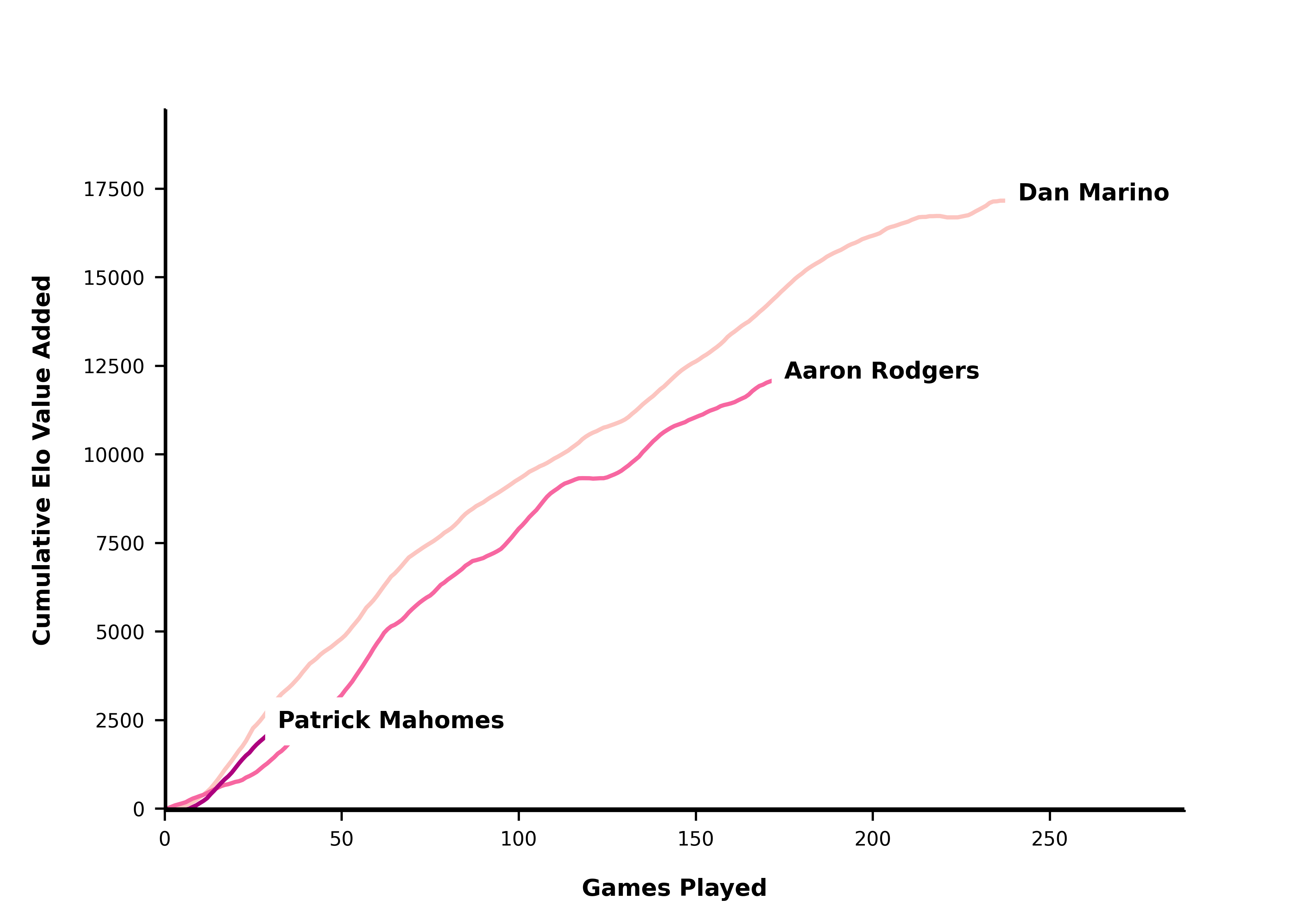
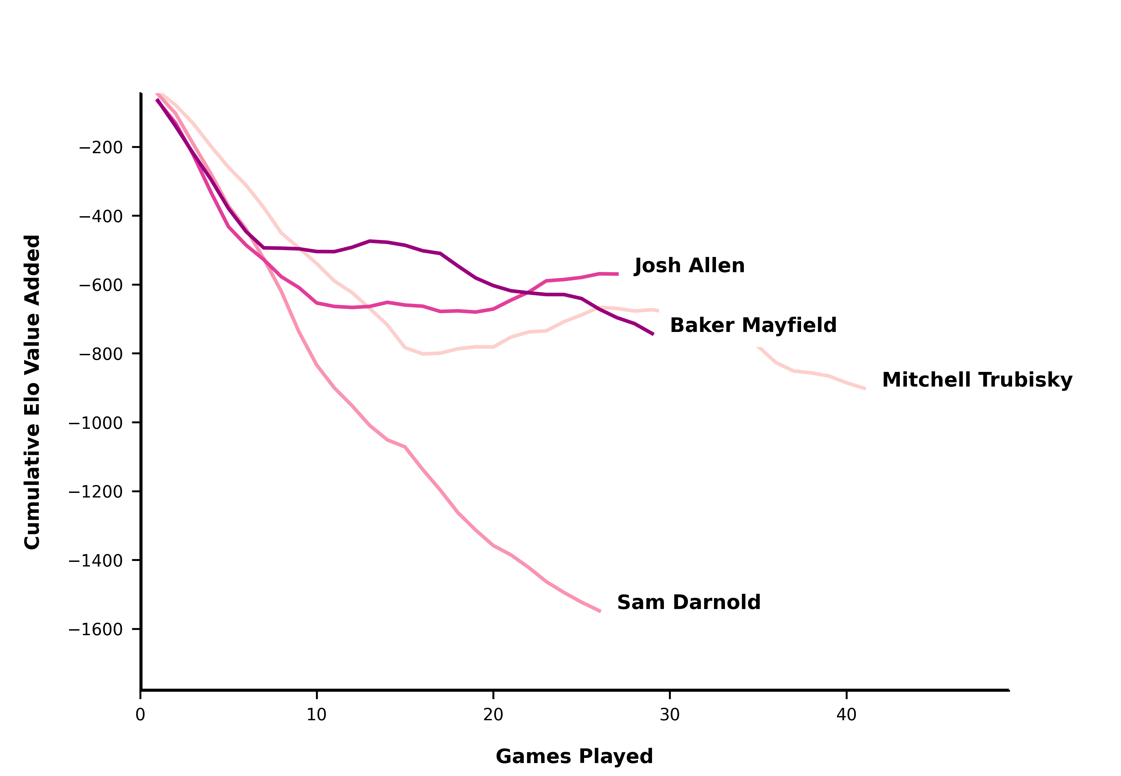
Josh Allen, not so much …
qb_list = ['Josh Allen', 'Sam Darnold', 'Mitchell Trubisky', 'Baker Mayfield']
create_qb_chart(qb_list)
plt.show()