Preface
In the NFL, practically everyone can beat anyone. So it often happens that games are tight until the very end and the winner is likely to have had some luck. Every year there are teams where you subjectively feel that they have lost or won particularly many of the aforementioned games.
In this post I will show off a very simple way to illustrate that by looking at how many snaps a team played with the nflfastR win probability (model with Vegas line) above a critical value (50%) more or less arbitrarily chosen by me and compare this value with the true win percentage.
Load nflfastR Play by Play and compute some helper columns
Since we want to compute true win percentage from nflfastR play-by-play data we have to do a little data wrangling before we can create the plot.
library(tidyverse)

# Parameter --------------------------------------------------------------------

season <- 2019
wp_limit <- 0.5

# Load the data ----------------------------------------------------------------

pbp <- readRDS(url(
  glue::glue("https://raw.githubusercontent.com/guga31bb/nflfastR-data/master/data/play_by_play_{season}.rds")
)) %>%
  filter(pass == 1 | rush == 1)

# Compute outcomes and win percentage ------------------------------------------

outcomes <- pbp %>%
  group_by(season, game_id, home_team) %>%
  summarise(
    home_win = if_else(result > 0, 1, 0),
    home_tie = if_else(result == 0, 1, 0)
  ) %>%
  group_by(season, home_team) %>%
  summarise(
    home_games = n(),
    home_wins = sum(home_win),
    home_ties = sum(home_tie)
  ) %>%
  ungroup() %>%
  left_join(
    # away games
    pbp %>%
      group_by(season, game_id, away_team) %>%
      summarise(
        away_win = if_else(result < 0, 1, 0),
        away_tie = if_else(result == 0, 1, 0)
      ) %>%
      group_by(season, away_team) %>%
      summarise(
        away_games = n(),
        away_wins = sum(away_win),
        away_ties = sum(away_tie)
      ) %>%
      ungroup(),
    by = c("season", "home_team" = "away_team")
  ) %>%
  rename(team = "home_team") %>%
  mutate(
    games = home_games + away_games,
    wins = home_wins + away_wins,
    losses = games - wins,
    ties = home_ties + away_ties,
    win_percentage = (wins + 0.5 * ties) / games
  ) %>%
  select(
    season, team, games, wins, losses, ties, win_percentage
  )

# Compute percentage of plays with wp > wp_lim ---------------------------------

wp_combined <- pbp %>%
  filter(!is.na(vegas_wp) & !is.na(posteam)) %>%
  group_by(season, posteam) %>%
  summarise(
    pos_plays = n(),
    pos_wp_lim_plays = sum(vegas_wp > wp_limit)
  ) %>%
  ungroup() %>%
  left_join(
    pbp %>%
      filter(!is.na(vegas_wp) & !is.na(posteam)) %>%
      group_by(season, defteam) %>%
      summarise(
        def_plays = n(),
        def_wp_lim_plays = sum(vegas_wp < wp_limit)
      ) %>%
      ungroup(),
    by = c("season", "posteam" = "defteam")
  ) %>%
  rename(team = "posteam") %>%
  mutate(
    wp_lim_percentage = as.numeric(pos_wp_lim_plays + def_wp_lim_plays) / as.numeric(pos_plays + def_plays)
  ) %>%
  select(season, team, wp_lim_percentage)

# Combine data and add colors and logos ----------------------------------------

chart <- outcomes %>%
  left_join(wp_combined, by = c("season", "team")) %>%
  filter(!is.na(wp_lim_percentage)) %>%
  mutate(diff = 100 * (win_percentage - wp_lim_percentage)) %>%
  group_by(team) %>%
  summarise_all(mean) %>%
  ungroup() %>%
  inner_join(
    nflfastR::teams_colors_logos %>% select(team_abbr, team_color, team_logo_espn, team_logo_wikipedia),
    by = c("team" = "team_abbr")
  ) %>%
  mutate(
    grob = map(seq_along(team_logo_espn), function(x) {
      grid::rasterGrob(magick::image_read(team_logo_espn[[x]]))
    })
  ) %>%
  select(team, win_percentage, wp_lim_percentage, diff, team_color, grob) %>%
  arrange(desc(diff))
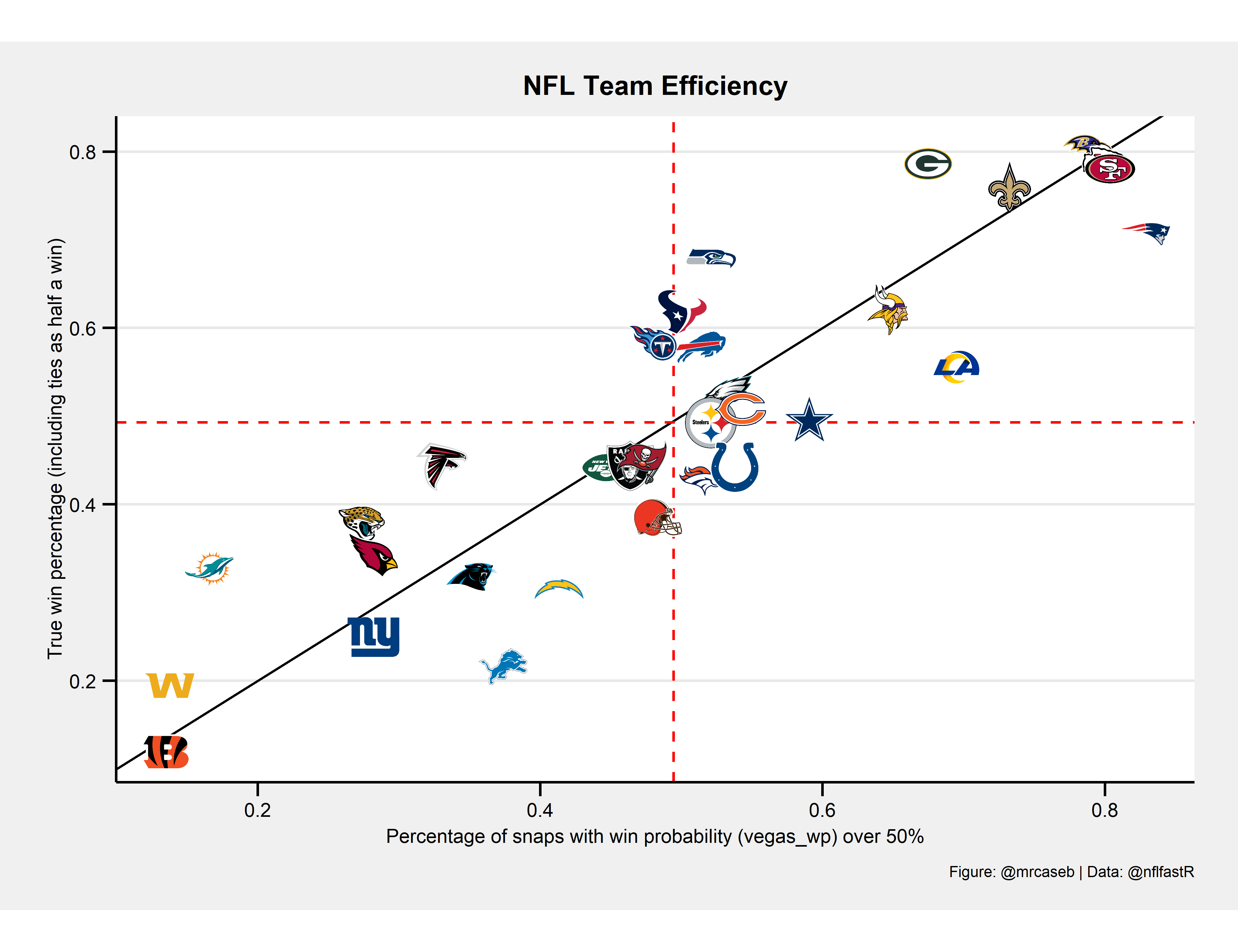
Create the plots
We will create two separate plots. A scatterplot comparing true win percentage with the percentage of plays with win probability > 50% and a barplot showing the difference between the above variables.
# Create scatterplot -----------------------------------------------------------
chart %>%
  ggplot(aes(x = wp_lim_percentage, y = win_percentage)) +
  geom_abline(intercept = 0, slope = 1) +
  geom_hline(aes(yintercept = mean(win_percentage)), color = "red", linetype = "dashed") +
  geom_vline(aes(xintercept = mean(wp_lim_percentage)), color = "red", linetype = "dashed") +
  ggpmisc::geom_grob(aes(x = wp_lim_percentage, y = win_percentage, label = grob), vp.width = 0.05) +
  labs(
    x = glue::glue("Percentage of snaps with win probability (vegas_wp) over {100 * wp_limit}%"),
    y = "True win percentage (including ties as half a win)",
    title = "NFL Team Efficiency",
    caption = "Figure: @mrcaseb | Data: @nflfastR"
  ) +
  ggthemes::theme_stata(scheme = "sj", base_size = 8) +
  theme(
    plot.title = element_text(face = "bold"),
    plot.caption = element_text(hjust = 1),
    axis.text.y = element_text(angle = 0, vjust = 0.5),
    legend.title = element_text(size = 8, hjust = 0, vjust = 0.5, face = "bold"),
    legend.position = "top",
    aspect.ratio = 1 / 1.618
  ) +
  NULL
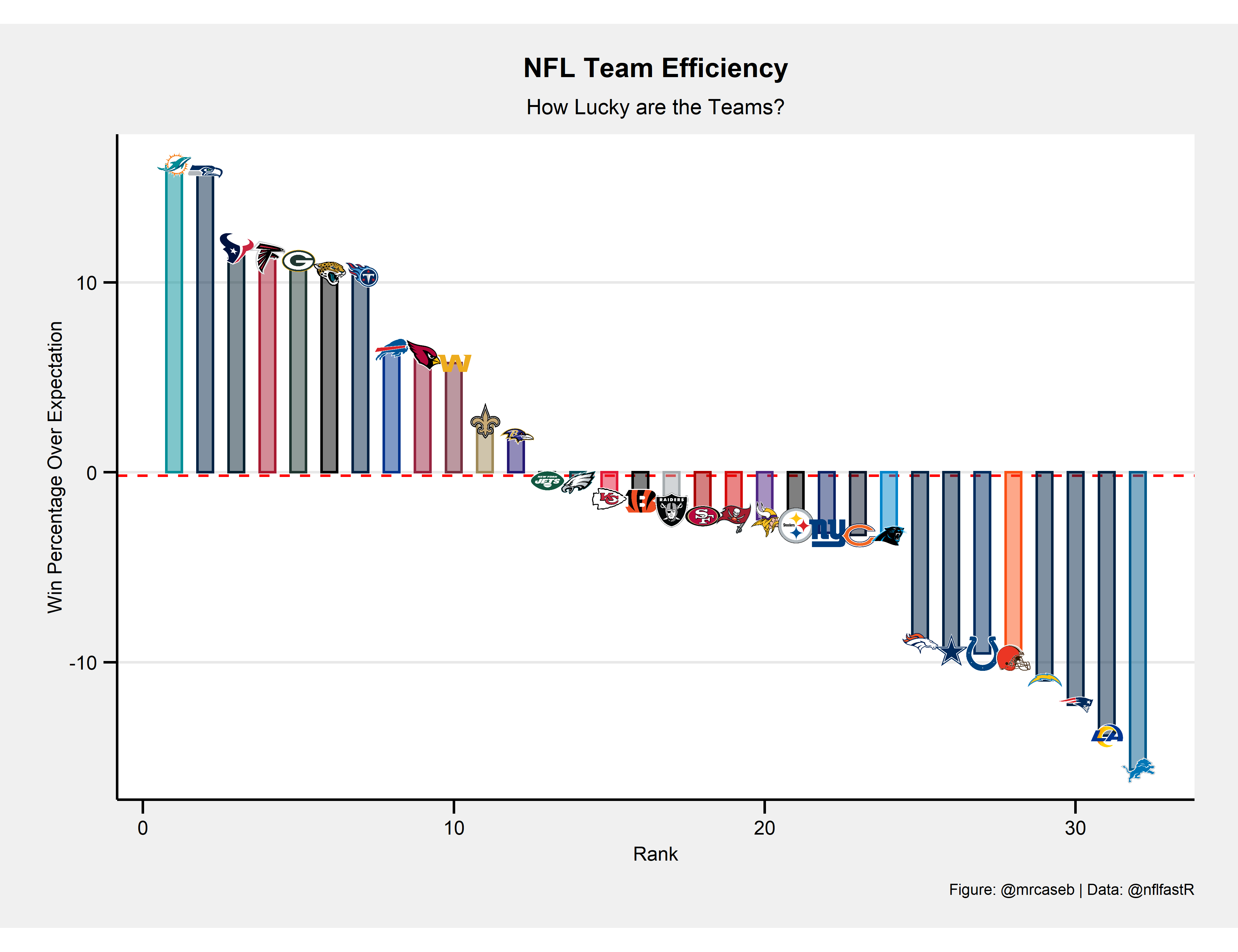
# Create bar plot  -------------------------------------------------------------
chart %>%
  ggplot(aes(x = seq_along(diff), y = diff)) +
  geom_hline(aes(yintercept = mean(diff)), color = "red", linetype = "dashed") +
  geom_col(width = 0.5, colour = chart$team_color, fill = chart$team_color, alpha = 0.5) +
  ggpmisc::geom_grob(aes(x = seq_along(diff), y = diff, label = grob), vp.width = 0.035) +
  # scale_x_continuous(expand = c(0,0)) +
  labs(
    x = "Rank",
    y = "Win Percentage Over Expectation",
    title = "NFL Team Efficiency",
    subtitle = "How Lucky are the Teams?",
    caption = "Figure: @mrcaseb | Data: @nflfastR"
  ) +
  ggthemes::theme_stata(scheme = "sj", base_size = 8) +
  theme(
    plot.title = element_text(face = "bold"),
    plot.caption = element_text(hjust = 1),
    axis.text.y = element_text(angle = 0, vjust = 0.5),
    legend.title = element_text(size = 8, hjust = 0, vjust = 0.5, face = "bold"),
    legend.position = "top",
    aspect.ratio = 1 / 1.618
  ) +
  NULL