Open Source Football: Neural Nets using R

Analytics Darkweb


library(reticulate)
library(tidyverse)

use_condaenv("r-tf-gpu", required = TRUE)


library(keras)

Before you proceed you will need to install Keras for R. In order to do that, I followed this guide. https://github.com/antoniosehk/keras-tensorflow-windows-installation

The following guide is heavily borrowed from the following Rstudio guide! https://tensorflow.rstudio.com/tutorials/beginners/basic-ml/tutorial_basic_regression/

Use the following lines to download the data if you need to.


seasons <- 2010:2019
pbp <- purrr::map_df(seasons, function(x) {
  readr::read_csv(
    glue::glue("https://raw.githubusercontent.com/guga31bb/nflfastR-data/master/data/play_by_play_{x}.csv.gz")
  )
})

Instead of throwing the kitchen sink at a problem, let’s choose some variables we think would influence yards after catch.


df <-
  pbp %>%
  filter(pass == 1) %>%
  mutate(
    pass_location = as.numeric(ifelse(pass_location == "middle", 1, 0)),
    roof = as.numeric(as.factor(roof))
    ) %>%
  select(yardline_100, down, ydstogo, shotgun, air_yards, yards_after_catch, qb_hit, pass_location, roof) %>%
  na.omit()

In this step you are converting your data frame into something Keras can injest.


set.seed(7)
sample <- sample.int(n = nrow(df), size = floor(.9*nrow(df)), replace = F)
train_df <- df[sample, ]
test_df  <- df[-sample, ]

train_labels <- train_df$yards_after_catch
test_labels <- test_df$yards_after_catch

train_df <- train_df %>% select(-yards_after_catch)
test_df <- test_df %>% select(-yards_after_catch)

column_names <- colnames(train_df)

train_df <- train_df %>% 
  as_tibble(.name_repair = "minimal") %>% 
  setNames(column_names) %>% 
  mutate(label = train_labels)

test_df <- test_df %>% 
  as_tibble(.name_repair = "minimal") %>% 
  setNames(column_names) %>% 
  mutate(label = test_labels)

Next we’ll use a little helper function to create the model, here we’re just doing a little toy model. No convolutions or anything too fancy. Just a little good ole fashioned brute force! Mostly because you should go read about different network types before you use them. :)


library(tfdatasets)

spec <- feature_spec(train_df, label ~ . ) %>% 
  step_numeric_column(all_numeric(), normalizer_fn = scaler_standard()) %>% 
  fit()

spec


-- Feature Spec --------------------------------------------------------------------------------------------------------------------------------------------------------------------------------------- 
A feature_spec with 8 steps.
Fitted: TRUE 
-- Steps ---------------------------------------------------------------------------------------------------------------------------------------------------------------------------------------------- 
The feature_spec has 1 dense features.
StepNumericColumn: yardline_100, down, ydstogo, shotgun, air_yards, qb_hit, pass_location, roof 
-- Dense features -------------------------------------------------------------------------------------------------------------------------------------------------------------------------------------


layer <- layer_dense_features(
  feature_columns = dense_features(spec), 
  dtype = tf$float32
)

build_model <- function() {
  input <- layer_input_from_dataset(train_df %>% select(-label))
  
  output <- input %>% 
    layer_dense_features(dense_features(spec)) %>% 
    layer_dense(units = 64, activation = "relu") %>%
    layer_dropout(.25) %>%
    layer_dense(units = 64, activation = "relu") %>%
    layer_dropout(.25) %>%
    layer_dense(units = 64, activation = "relu") %>%
    layer_dropout(.25) %>%
    layer_dense(units = 1) 
  
  model <- keras_model(input, output)
  
  model %>% 
    compile(
      loss = "mse",
      optimizer = "adam",
      metrics = list("mean_absolute_error")
    )
  
  model
}

early_stop <- callback_early_stopping(monitor = "val_loss", patience = 20)

print_dot_callback <- callback_lambda(
  on_epoch_end = function(epoch, logs) {
    if (epoch %% 20 == 0) cat("\n")
    cat(".")
  }
)  

model <- build_model()

summary(model)


Model: "model"
______________________________________________________________________
Layer (type)           Output Shape   Param # Connected to            
======================================================================
air_yards (InputLayer) [(None,)]      0                               
______________________________________________________________________
down (InputLayer)      [(None,)]      0                               
______________________________________________________________________
pass_location (InputLa [(None,)]      0                               
______________________________________________________________________
qb_hit (InputLayer)    [(None,)]      0                               
______________________________________________________________________
roof (InputLayer)      [(None,)]      0                               
______________________________________________________________________
shotgun (InputLayer)   [(None,)]      0                               
______________________________________________________________________
yardline_100 (InputLay [(None,)]      0                               
______________________________________________________________________
ydstogo (InputLayer)   [(None,)]      0                               
______________________________________________________________________
dense_features_1 (Dens (None, 8)      0       air_yards[0][0]         
                                              down[0][0]              
                                              pass_location[0][0]     
                                              qb_hit[0][0]            
                                              roof[0][0]              
                                              shotgun[0][0]           
                                              yardline_100[0][0]      
                                              ydstogo[0][0]           
______________________________________________________________________
dense (Dense)          (None, 64)     576     dense_features_1[0][0]  
______________________________________________________________________
dropout (Dropout)      (None, 64)     0       dense[0][0]             
______________________________________________________________________
dense_1 (Dense)        (None, 64)     4160    dropout[0][0]           
______________________________________________________________________
dropout_1 (Dropout)    (None, 64)     0       dense_1[0][0]           
______________________________________________________________________
dense_2 (Dense)        (None, 64)     4160    dropout_1[0][0]         
______________________________________________________________________
dropout_2 (Dropout)    (None, 64)     0       dense_2[0][0]           
______________________________________________________________________
dense_3 (Dense)        (None, 1)      65      dropout_2[0][0]         
======================================================================
Total params: 8,961
Trainable params: 8,961
Non-trainable params: 0
______________________________________________________________________

Next let’s run the model and see how it does!


history <- model %>% fit(
  x = train_df %>% select(-label),
  y = train_df$label,
  epochs = 500,
  batchsize = 64,
  validation_split = 0.2,
  verbose = 0,
  callbacks = list(print_dot_callback, early_stop)
)


....................
.................

Now to check the results!

Here we visualize how our nnet trained over our epochs. We define epochs here since we had some early stopping.


library(ggplot2)
history$params$epochs <- length(history$metrics$loss)

plot(history)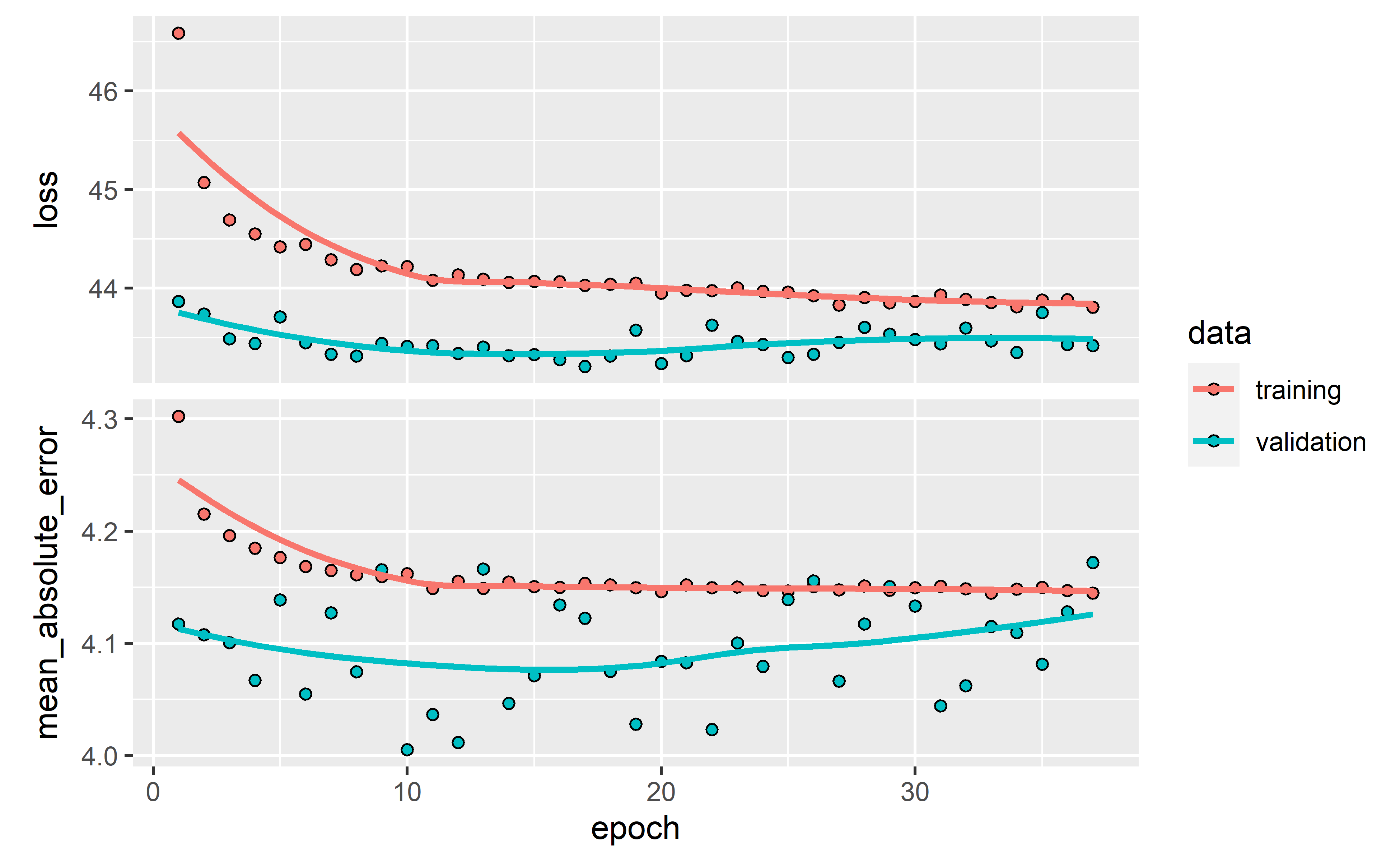


test_predictions <- model %>% predict(test_df %>% select(-label))

Next we can take a look at the mean absolute error and loss from our model on the test set.


c(loss, mae) %<-% (model %>% evaluate(test_df %>% select(-label), test_df$label, verbose = 0))

loss


[1] 46.37026

mae


[1] 4.239087


test_predictions <- test_predictions %>% as.data.frame()

test_predictions %>% ggplot(aes(V1)) + geom_density()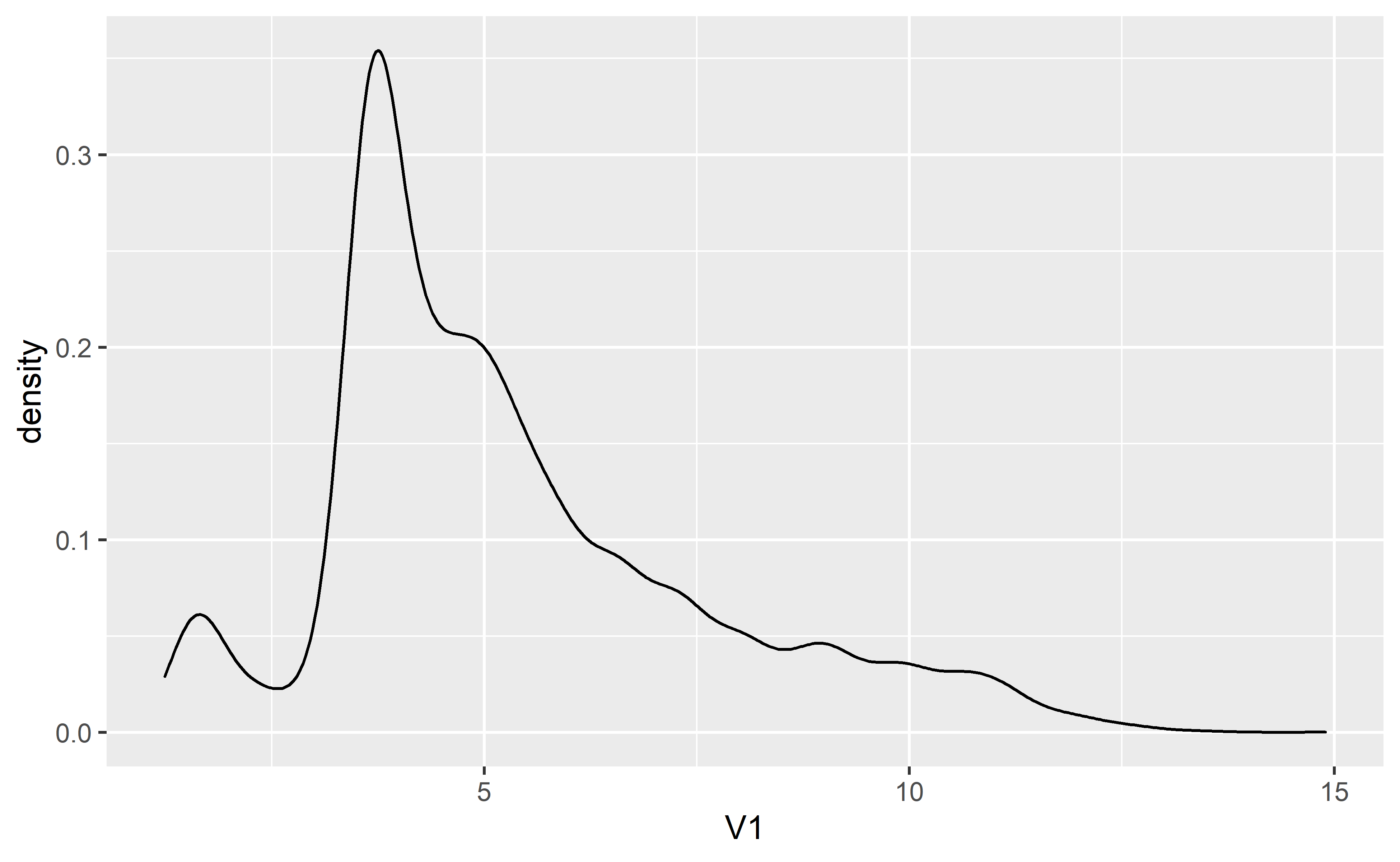

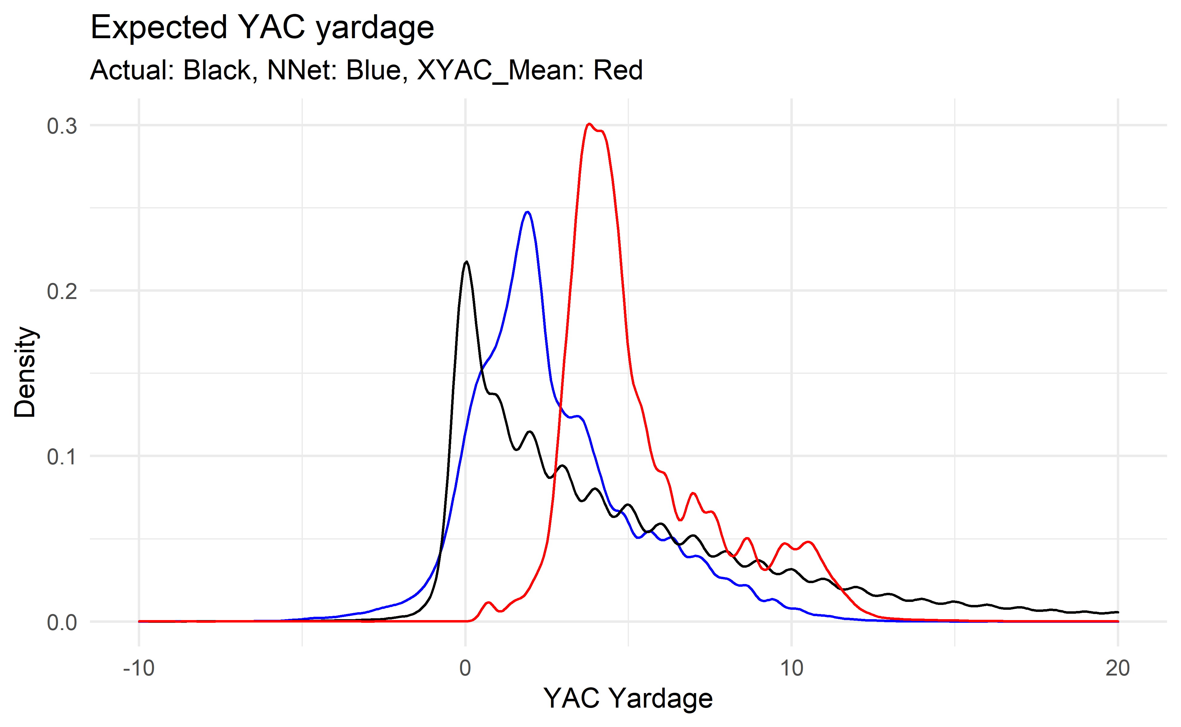
Lastly, let’s visualize our trained model versus both actual YAC yardage and nflfastR’s XYAC mean yards model.


df <-
  pbp %>%
  filter(pass == 1) %>%
  mutate(
    pass_location = as.numeric(ifelse(pass_location == "middle", 1, 0)),
    roof = as.numeric(as.factor(roof))
  ) %>%
  select(yardline_100, down, ydstogo, shotgun, air_yards, yards_after_catch, qb_hit, pass_location, roof, xyac_mean_yardage) %>%
  na.omit()

train_df <- df %>% 
  as_tibble(.name_repair = "minimal") %>% 
  setNames(colnames(df)) %>% 
  mutate(label = yards_after_catch)

test_predictions <- model %>% predict(train_df %>% select(-label))

test_predictions <- test_predictions %>% as.data.frame()

df <- 
  cbind(df, test_predictions)

df %>%
  ggplot() + 
  geom_density(aes(V1), color = "blue") + 
  geom_density(aes(yards_after_catch)) + 
  geom_density(aes(xyac_mean_yardage), color = "red") +
  xlim(c(-10, 20)) + 
  theme_minimal() + 
  labs(
    title = "Expected YAC yardage",
    x = "YAC Yardage",
    y = "Density",
    subtitle = "Actual: Black, NNet: Blue, XYAC_Mean: Red"
    
  )

There you have it, your own little nnet done completely in R using the Keras/tensorflow backend.

Neural Nets using R

Corrections

Reuse

Citation